New Global Formulation for a Bilateral based Stereo Matching Algorithm

New Global Formulation for a Bilateral based Stereo

Matching Algorithm

Doaa A. Altantawy

Engineering Department Faculty of Engineering

Mansoura University Mansoura, Egypt

Marwa Obbaya

Engineering Department Faculty of Engineering

Mansoura University Mansoura, Egypt

Sherif S. Kishk

Engineering Department Faculty of Engineering

Mansoura University Mansoura, Egypt

ABSTRACT

In this paper, a new hybrid local-global stereo matching algorithm (BFGc) is proposed. BFGc makes the maximum benefit from both the introduced local and the global approaches representing the main two stage of the algorithm. Globally, a new energy formulation of the stereo problem in segment domain is proposed which basically depends on the reliability of the disparity estimates results from the adopted local approach, unlike what is typical in global methods. For increasing reliability of the local approach, a new gradient masks is supporting the adopted similarity measure and Bilateral filter, with its edge preserving sense, is adopted for more proper disparity assignment. In segment domain, a plan fitting technique is introduced which aims at inferring all valid planes in disparity space and producing a good initialization for the global optimization space which aims at assigning memberships to the these planes to all pixels in the reference image. The experimental results on the Middleburry dataset demonstrate that our approach stands as a strong candidate with the modern stereo matching algorithms.

General Terms

Computer vision, Stereo vision, Digital image processing

Keywords

Stereo matching, Self-adapting similarity measure, Color segmentation, Graph cuts

1.

INTRODUCTION

The basic problem with a stereo matching algorithm is to identify corresponding points in two images that are recorded from slightly different perspectives [1]. To simplify the search for correspondences, the two images are aligned with respect to each other, i.e. rectified. Image rectification is the process of transforming two images such that their epipolar lines are horizontal and parallel. Disparity describes the difference in location of the corresponding pixels and it is often considered as a synonym for inverse depth. Due to the ill-posed nature of the stereo matching problem, the recovery of accurate disparity still remains challenging, especially in textureless regions, disparity discontinuous boundaries and occluded areas.

An excellent review of stereo algorithms is detailed in [1] where the stereo matching algorithms are categorized into two major classes. The first class is local (area-based) algorithms, which generally use some kind of statistical correlation between color or intensity patterns in the local support windows. By using local support windows, image ambiguity

is reduced efficiently while the discriminative power of the similarity measure is increased. However, the assumption that all pixels in a support window are from similar depth in a scene and, therefore, they have similar disparities, leads to disparity discontinuous boundaries and this may result in the ‘foreground-fattening’ phenomenon. Moreover, they are exposed to many failure sources, such as occlusions or variations of intensity between the two images due to light variations, non Lambertian surfaces and camera electronics which lead to many false matches. However, Local methods [2, 3] are in general fast and can be used in real time applications.

Global methods, as the second class, try to overcome the previous problems through a definition of a global model of observed scene to minimize a global cost function with explicit smoothing assumptions which suit the stereo problem. Textureless regions can be handled effectively in this framework. However, enforcing the smoothness usually tends to sacrifice discontinuities in disparity. Thus, an efficient discontinuity preserving smoothness constraint must be considered. Popular global methods use graph cuts [4, 5] or belief propagation [6, 7] to minimize the energy function. An extensive performance comparison of graph cuts and belief propagation methods is made in [8].

Recently, segment-based methods [5-7] have attracted attention due to their good performance on handling boundaries and textureless regions. They are based on the assumption that the scene structure can be approximated by a set of non-overlapping planes in the disparity space and that each plane is coincident with at least one homogeneous color segment in the reference image. In fact, nearly all of the top-ranked methods in the Middlebury benchmark use image segmentation in some way [5-7, 9-11]. Segment-based stereo matching generally performs four consecutive steps [5, 6, 10]. First, segment the reference image using robust segmentation method; second, get initial disparity map using local match method; third, a plane fitting technique is employed to obtain disparity planes; finally, an optimal disparity plane assignment is approximated using belief propagation or graph cut optimization method.

filter, i.e. Bilateral filter [12]. Secondly, in segment domain, stereo problem is turned to an energy minimization function which aims at assigning memberships to the valid initial linear disparity planes to all pixels in the reference image. A new energy function is formulated with the use of graph cuts that depends on the reliability of the initial obtained disparity planes, unlike to what is common in most of the global algorithms that depends on the matching score of the segments’ pixels [5,6,10].

The remainder of this paper is organized as follows. Section 2 indicates related work and motivation. The color segmentation process and extracting the most reliable linear disparity planes are demonstrated respectively in Sections 3, 4. The new stereo formalization for final disparity plane labeling using graph is shown in Section 5. Finally the experimental results and conclusion are indicted in Section 6, 7 respectively.

2.

RELATED RESEARCHES

To get over the problems of the early standard local algorithms in dealing with edge fattening problem when the support window overlaps a disparity discontinuity, an appropriate support window should be selected for each pixel adaptively. To this end, many methods have been proposed. They can be roughly divided into several categories according to their techniques. In [13-17], adaptive-window methods are proposed trying try to find an optimal support window for each pixel by changing the size and shape of a window adaptively. In [13], Kanade and Okutomi proposed selecting an appropriate window by evaluating the local variation of intensity and disparity. However, the shape of a support window is constrained to a rectangle, which is not appropriate for the pixels near arbitrarily shaped depth discontinuities besides the high computational cost of this technique. Boykov et al. [14], on the other hand, tried to choose an arbitrarily shaped connected window by performing plausibility hypothesis testing and computing a correct window for each pixel.

Multiple-window methods represent another category in enhancing the performance of the local methods. In [15], [16], [17] an optimal support window is selected among the pre-defined multiple windows, which are located at different positions with the same shape. The correlation with nine different windows for each pixel is performed by Fusiello et al. in [15] and the disparity with the smallest matching cost is retained. In addition, Kang et al. [17] examines all windows containing the pixel of interest. To get over the problems of the previous mentioned methods in finding the optimal support window with an arbitrary shape and size [13-17], adaptive support weight approaches have been introduced [2,3,11,18] trying to assign appropriate support-weights to the pixels in a support window while fixing the shape and size of a local support window. These methods deal with the pixels near depth discontinuities more effectively than the methods mentioned above .Such methods were pioneered by Yoon and Kweon [19] at which the weights depend on both color and spatial distance to the central pixel of the window. Many variations of the Yoon and Kweon method have been introduced since then. Segment-based approaches [11, 20] represent a new trend in local adaptive techniques by employing information obtained from the application of segmentation within the weight cost function in order to increase the robustness of the matching process. Performing the aggregation of the adaptive weight algorithms with an edge preserving filter represent a new trend in the adaptive local methods like using the Guided filter in [21]. It is worth

noting that cost volume filtering represent one of the best local methods for the Middlebury dataset with a good edge preserving behavior but may suffer with textureless regions which have different characteristics from edges. For more trends in local adaptive methods, the reader referred to read [22] for batch-based methods, [2, 3, 23, 24] for accelerated local versions.

Most modern approaches frame the problem of the stereo matching utilizing global optimization techniques such as [5-7, 9, 10]. Boykov et al. [4] proposed a stereo algorithm that applies graph cuts to optimize a cost function consisting of a data term that measures the pixel dissimilarity and a smoothness term that puts a constant penalty on neighboring pixels assigned to different disparities. Then, Kolmogorov and Zabih extended this work for handling occlusion in [25]. Recently, the segmentation constraint is used in conjunction with different optimization schemes, graph cuts is one of them.

In comparison to the proposed algorithm BFGc in this paper, the slanted-plane method proposed by Birchfield and Tomasi [26] is considered as being similar in the sense. They formulate the correspondence problem in two steps. First, they estimate a set of plane models that correspond to different depth surfaces occurring in the scene. In the second step, they then assign each pixel to exactly one of those planes. Then, this model is extended to different slanted plane models techniques which combine region-based matching with graph-based optimization. These slanted-plane models [5-7,10,27] include typically a robust data term scoring the assigned plane in terms of a matching score induced by the plane on the pixels contained in the segment in addition to a smoothness term expressing the belief that the planes assigned to adjacent segments should be similar.

In this work, unlike to the previous common slated-plane models, the proposed segment-based method employs a new data term based on the reliability of the initial estimated planes. Hence, BF is used for cost volume filtering for an edge preserving sense in initial disparity assignment. In addit-

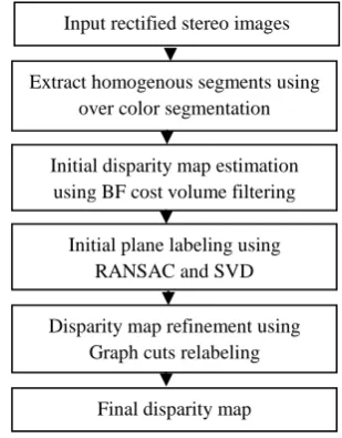
Fig. 1:The block diagram of the proposed BFGc algorithm.

Input rectified stereo images

Extract homogenous segments using over color segmentation

Initial disparity map estimation using BF cost volume filtering Initial plane labeling using

RANSAC and SVD

Disparity map refinement using Graph cuts relabeling

Table 1. Average error percentages according to Middlebury benchmark for initial disparity map using similarity measure in Eqn.1 using different gradient masks.

Gradient mask

Tsukuba Venus Teddy Cones

Non-occ All Disc

Non-occ All Disc

Non-occ All Disc

Non-occ All Disc (a) 20.7 22.5 25.4 33 34.1 38.3 37.7 44.1 44.7 21.3 30.2 31.9

(b) 18.9 20.7 25.8 32.7 33.8 38 37.8 44.2 45 21.3 30.2 32.4

(c) 18.8 20.6 26 32.1 33.3 38.4 37.6 44 45.2 21.1 30 32.4

(d) 12.4 14.4 24.4 24.6 25.9 37.7 27 34.5 37.8 15.2 24.9 28.8

Procedure: (a) the simplest gradient masks as , (b) Prewitt gradient masks, (c) Sobel gradient masks and finally (d) the proposed gradient masks as in Eqn. 4. The bad pixel percentages is computed for (1) non occluded pixels only (Nonocc), (2) all pixels (All) and (3) pixels that are close to disparity discontinuity (Disc).

ion, for more reliable linear disparity planes, RANSAC [28] and SVD are deployed. Moreover, the disparity plane estimation process is utilized after across-validation test and a judging rule for extracting the most reliable disparity planes.

3.

COLOR SEGMENTATION

The proposed BFGc approach is one of the segment-based methods at which a disparity planar or surface model is assigned to one homogeneous color segment instead of assigning a proper disparity value to individual pixel one by one, so these homogenous regions have to be extracted from the reference image. Hence, over segmentation techniques should be adopted taking into consideration that their success in the disparity estimation process will depend on the ability of these algorithms to delineate precisely the objects' outlines. The mean-shift color segmentation [29], used in many modern stereo algorithms, is applied here which allows the accurate localization of depth discontinuities and handles Large textureless regions.

4.

DISPARITY PLANES EXTRACTION

For the estimation of all the possible disparity planes, a sparse initial disparity map must be computed firstly through local matching analysis. Secondly, the initial plane parameters from each color segment (while skip very small segments) are estimated for getting a planar model.

4.1

Local matching approach in pixel

domain

A local approach should be adopted in order to get an initial disparity map and this approach should define a matching cost (or a dissimilarity measure) with an aggregation window or method. The proposed local approach consists of three steps: first, cost volume construction using a self-adapting similarity measure; second, cost volume filtering using Bilateral filter; finally, disparity level selection by using WTA (winner-take-all) strategy.

4.1.1

Matching cost computation

Given two rectified stereo pairs , the correspondence between a pixel in the reference image and a pixel

in the matching image is given by

, where the disparity can take any discrete value from the disparity levels interval

. Let denote the matching cost for the pixel in image with disparity level and it is defined

as being a weighted sum of gradient and color

differences as:

(1)

(2)

(3)

Where is the optimal weight between and and

it is determined by maximizing the number of reliable correspondences that are filtered out by applying a cross-checking test (comparing left-to-right and right-to-left disparity maps). and denote the gradient in x-direction and y-direction respectively. Finally, is a 3 × 3 surrounding window at position .

For getting the gradient components, a 7-tab gradient mask is proposed according to [30] as in Eqn.4. These gradient masks provide more effectiveness than the other common gradient masks, such as Sobel, Prewitt and the simplest gradient masks as , in extracting more reliable disparity estimates according to Middleburry evaluation [31] and these results are indicated in Table 1.

(4)

4.1.2

Matching cost filtration and disparity

assignment:

consists of has two filter kernels, a spatial and a range kernel, for calculating the spatial and intensity range distance between the center pixel and its neighbors. Hence, the matching cost for a pixel at a disparity level (for simplicity, single letters are used for denoting pixels) is expressed as

where is the kernel window which is centered at pixel . The standard deviation parameter is responsible for control of decrement of weight in spatial domain, whereas the parameter controls the decrement of weight in intensity range domain. denotes the Euclidean distance between pixels and .

The idea behind using the weights of the BF for cost volume filtration is that the weight assigned to each pixel in a specific window is a representation of the probability that this pixel and the central pixel of the window have the same disparity. The spatial weighting decreases with the Euclidean distance, which makes the pixels cost value less influential on the final cost result and the intensity weighting ensures that the pixels whose initial cost value significantly differ from the central pixel’s have less influence on .

After the matching cost volume filtration, the Winner-Takes-All strategy (WTA) is applied to choose the best disparity value for each pixel as

(7)

where represents the set of all allowed disparities in the interval .

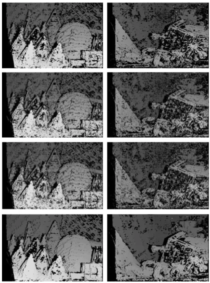
In Table 2, the computational results of initial disparity maps and cross-check maps after BF cost volume filtering is indicated using the proposed gradient masks in comparison with other gradient masks which prove the effectiveness of the proposed gradient masks with BF technique in extracting more reliable disparity estimates. For supporting visual results, Fig. 2 indicates the cross-check maps under the same cases at which dark point means an outlier for Teddy and Cones.

4.2

Initial plane fitting from single segment

The initial disparity map is used to initialize the planar equation of each segment as

where , , are the plane parameters and is the

corresponding disparity of the image pixel . ( , , ) is the least square solution of a linear system formulated as

where the row of is , the element in is the initial disparity value and is the plane parameters , , . This least square solution is obtained using SVD as in [10].

The least square solution can be biased by unreliable initial disparity estimates. Hence, the following two procedures are

Table 2. Bad pixels percentage according to Middleburry evaluation for initial disparity map and cross-check map

BF Cost volume filtering technique

Initial disparity

map Cross-check map

Non-occ All Disc

Non-occ All Disc

(a)

Tsukuba 13 15 21.6 24.9 26.8 36.7 Venus 20.9 22.2 33.4 31.6 32.8 44.3 Teddy 24.6 32.4 37.8 38.7 45.1 51.6 Cones 12.4 22.4 25.1 26.3 34.8 42.4

(b)

Tsukuba 13.1 15 23 24.6 26.5 38.2 Venus 22.7 24 34.6 34.4 35.5 44.4 Teddy 27.9 35.4 40.6 42.2 48.2 53.7 Cones 15.4 25 28.7 28.5 36.8 44.1

(c)

Tsukuba 13.7 15.6 23.2 25.5 27.3 38.1 Venus 24.7 25.9 34.4 37.2 38.3 45.1 Teddy 30.1 37.4 41.4 45 50.8 54.8 Cones 17 26.4 29.5 30.5 38.5 44.9

(d)

Tsukuba 8.48 10.6 21.6 15.4 17.5 34

Venus 15.7 17.1 34 23.8 25.1 41.6

Teddy 17.5 26.1 32.3 27.9 35.4 43.3

Cones 9.24 19.6 22.9 20 29.2 36.7 Procedure: (a) the simplest gradient masks as

, (b) Prewitt gradient masks, (c) Sobel gradient masks and finally (d) the proposed gradient masks as in Eqn. 4.

adopted for so only pixels with reliable initial disparity estimation are included to form the previous linear system

as following:

 With local methods, reliable disparity estimates can’t be provided especially in textureless and occluded regions, so the initial rough disparity map after cost volume filtering will contain a large number of outliers especially in these regions. The conventional way to exclude these outliers is performing a left-right consistency check. Hence, let pixel

in the matching image is the correspondence of pixel

in the reference image based on the initial disparity , and let be the initial disparity of pixel in the matching image. If , we consider pixel as an outlier.

 RANSAC [32] is applied over the most reliable segments, i.e. contain 50% of its pixels inliers after the cross-validation test, to select the most proper pixels to be included for least square solution of using SVD.

5.

FINAL DISPARITY PLANE

LABELING USING GRAPH CUTS

In order to refine the obtained disparity map, disparity plan assignment is formalized as an energy minimization problem in segment domain and will be solved using graph cuts in which each node of the graph corresponds to a different segment, i.e., labeling each segment with its corresponding disparity plane.

Let be the set of disparity planes parameters (labels), and be the color segments of the reference image. The goal here is to find a labeling that assigns each segment to its plane label by minimizing an energy function ; this energy function combine a data cost that

represent a penalty for assigning a segment a label and a smoothing cost that helps to penalize the discontinuities in plane labels of neighboring segments and finally an occlusion cost to punish occlusion in each segment

In most of the state-of-the-art algorithms, such as [5,6,10], the matching cost in Eqn. 1 are used as the data term for non-occluded pixels, but it is not that simple process in calculations. Here, a new data term will be applied as

where is a scaling coefficient, represents the disparity of the pixel after plane fitting with label , is the initial disparity for the same pixel , is the number of non-occluded pixels that has the same initial disparity as the disparity after plane fitting, is the number of non-occluded pixels inside the segment and is the set of occluded pixels considered as the number of detected unreliable pixels in the segment .

The following smoothing cost is used to judge adjacent segments relationship:

where represents a set of all adjacent segments, are neighboring segments, is a smoothing coefficient, is the common border length (number of common border pixels) between segments and is a color similarity measure between the segments and it is defined in Eqn. 12. The basic idea behind weighting the smoothness penalty by the color similarity measure is that two segments showing similar color are considered as more likely to originate from the same real-world surface than two segments of completely different color.

where is the componentwise summed up RGB values of pixels inside segment divided by their number. For identical mean color values, the color similarity function returns a value of 0.5, whereas for color differences larger or equal to 255, it gives a value of 0. Hence, the costs of assigning two neighboring segments of similar color to different disparity planes are therefore higher than separating two segments of low color similarity.

For the occlusion energy function is utilized to punish the occlusion pixels in segment, the expression of the occlusion energy function is

A graph G is then reconstructed and graph cuts is applied to approximate the global minimum of our energy function. Here, the graph nodes represent segments instead of pixels, and the label set is composed of all the estimated disparity planes instead of all possible discrete values in the disparity range.

6.

EXPERMINTAL RESULTS

To evaluate the performance of the proposed BFGc approach, we employ four standard image pairs providing a variety of cases, including disparity discontinuous boundaries, textureless and occluded regions. The commonly-accepted Middlebury benchmark [31] is used to evaluate all the proposed method steps. Herein, a disparity value is defined to be erroneous if the absolute difference from the ground truth is more than one [1]. The percentage of bad matching pixels is computed for (1) non occluded pixels only (Nonocc), (2) all pixels (All) and (3) pixels that are close to disparity discontinuity (Disc).

Table 3. The percentage of bad pixels for Middlebury datasets at the different stages of the proposed BFGc algorithm is indicated.

Procedure steps: (1) initial disparity map using the similarity measure in Eqn. 1, (2) Initial disparity map using BF cost volume filtering, (3) Disparity map after plane fitting and (4) Final disparity map after graph cuts labeling.

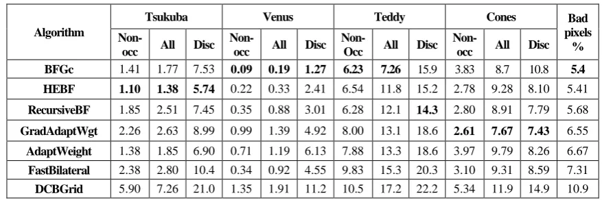
Table 4. Results of the most common BF based stereo matching algorithms with the proposed BFGc.

besides the plane fitting technique demonstrate their role, that can’t be ever neglected, in extracting the most reliable disparity planes for the final labeling using graph cuts. In Table 4, a comparison is set between the proposed BFGc approach and different common stereo matching algorithm based on BF. AdaptWeight is the first introduced adaptive weight algorithm in [19] by Yoon and Kweon which propose using BF in the initial matching process between the stereo images with SAD similarity measure with very large window

which increases the computation cost of the algorithm. In [18], De-Maeztu et al. introduce the same technique of AdaptWeight but with truncated based gradient similarity measure which proves effectiveness over the original AdaptWeight. At DCBGrid reported by Richardt et al. [3], the cost volume is smoothed with a fast approximation of the bilateral filter. Due to this approximation, huge amounts of memory would be required when applied to full-color (e.g. RGB) stereo images. Therefore, [3] is limited to grayscale input images, giving poor results at disparity boundaries as indicated from the results of the bad pixels percentage in disparity discontinuities. RecursiveBF and FastBilateral proposed in [24], [23] respectively represent a speeded up versions of BF at cost of the quality of the original BF and for the indicated results, different refinement steps were adopted. HEBF [2] is another speeded up version of BF used for cost volume filtering and is finished by several post processing steps for disparity refinement and occlusion handling. In addition, HEBF shows a faster and better performance than RecursiveBF and FastBilateral as shown from their results. Moreover, HEBF shows a strong candidate

performance to ours. However, the proposed BFGc shows an optimum performance in dealing with textureless regions. Fig. 4 shows visual results of the obtained disparity maps for Middleburry datasets according to the proposed BFGc. Experimentally, the parameters are chosen as following: for the matching cost ( ), for Mean shift segmentation ( ), for Bilateral filter (

), and finally for graph cuts (

)

7.

CONCLUSION

This work presents a hybrid-local global segment-based disparity map estimation technique (BFGc). According to the Middleburry benchmark, the proposed method provides very low percentage of bad pixels in the estimated disparity map especially in the conventionally difficult areas such as textureless regions, disparity discontinuous boundaries and occluded portions. Also, the best results are obtained with textureless regions with a disparity map very similar to the ground truth as indicated from the Venus scene achieving a 3rd rank among more than 160 submission. This effectiveness is achieved in two domains, in pixel domain at which the proposed gradient masks increase the ability of the matching measure and BF cost volume filtering in extracting more reliable disparity estimates. Secondly, the introduced plane extraction technique in segment domain helps the new energy formulation of the stereo problem for getting more reliable final disparity maps.

Procedures

Tsukuba Venus Teddy Cones Non

occ All Disc Non

occ All Disc Non

occ All Disc Non

occ All Disc (1) 13 14.9 23.1 25.3 26.6 35.8 27.5 35.6 38.9 16.4 25.7 30.7

(2) 8.48 10.6 21.6 15.7 17.1 34 17.5 26.1 32.3 9.24 19.6 22.9

(3) 4.93 5.91 14.5 2.91 3.81 17.2 8.48 14.6 20.5 5.53 14 13.6

(4) 1.41 1.77 7.53 0.09 0.19 1.27 6.23 7.26 15.9 3.83 8.7 10.8

Algorithm

Tsukuba Venus Teddy Cones Bad pixels

%

Non-occ All Disc

Non-occ All Disc

Non-Occ All Disc

Non-occ All Disc BFGc 1.41 1.77 7.53 0.09 0.19 1.27 6.23 7.26 15.9 3.83 8.7 10.8 5.4 HEBF 1.10 1.38 5.74 0.22 0.33 2.41 6.54 11.8 15.2 2.78 9.28 8.10 5.41

RecursiveBF 1.85 2.51 7.45 0.35 0.88 3.01 6.28 12.1 14.3 2.80 8.91 7.79 5.68

GradAdaptWgt 2.26 2.63 8.99 0.99 1.39 4.92 8.00 13.1 18.6 2.61 7.67 7.43 6.55

AdaptWeight 1.38 1.85 6.90 0.71 1.19 6.13 7.88 13.3 18.6 3.97 9.79 8.26 6.67

FastBilateral 2.38 2.80 10.4 0.34 0.92 4.55 9.83 15.3 20.3 3.10 9.31 8.59 7.31

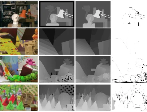
Fig. 3: Different stages of the proposed BFGc for Venus and Teddy respectively from top to bottom. From left to right; Results after initial disparity map using the similarity measure in Eqn. 1, Initial disparity map after cost volume filtering using BF, Disparity map after plane fitting, and Finally, the resulting disparity maps after graph cuts labeling.

8.

REFRENCES

[1] Scharstein, D. and Szeliski, R. 2002. A taxonomy and evaluation of dense two-frame stereo correspondence algorithms, Int. J. Comput. Vis. 47 (1/2/3) (2002) 7–42. [2] Yang, Q. 2013. Hardware-efficient bilateral filtering for

stereo matching. IEEE Trans. on PAMI, 36(5) 1026 - 1032 .

[3] Richardt, C., Orr, D., Davies, I., Criminisi, A., and Dodgson, N. A. (2010). Real-time spatiotemporal stereo matching using the dual-cross-bilateral grid. In Proc. Of ECCV , 510-523. Springer Berlin Heidelberg.

[4] Boykov, Y., Veksler, O. and Zabih, R.2001. Fast Approx- imate Energy Minimization via Graph Cuts. IEEE Trans. PAMI. 23 (2001)1222-1239.

[5] Hong, L. and Chen, G. 2004. Segment-Based Stereo Matching Using Graph-Cuts. In Proc. of CVPR, (1)74- 81.

[6] Klaus, A., Sourmann, M. and Karner, K. 2006. Segment- Based Stereo Matching Using Belief Propagation and a Self Adapting Dissimilarity Measure. In Proc. Of ICPR, 15-18

[7] Yang, Q. , Wang, L., Yang, R., Stewenius, H. and Nister, D.2009. Stereo Matching with Color-Weighted Correlation, Hierarchical Belief Propagation, and Occlusion Handling. IEEE Trans. on PAMI, (3) 492-504. [8] Tappen, M. and Freeman, W.2003. Comparison of Graph Cuts with Belief Propagation for Stereo. In Proc. Of ICCV, (1)508-515.

[9] Bleyer, M., Rother, C., Kohli, P., Scharstein, D. and Sinha, S. 2011. Object stereo - joint stereo matching and object segmentation. In Proc. Of CVPR, 3081-3088

[10] W. Daolei, K. Lim, Obtaining depth map from segment-based stereo matching using graph cuts, J. Vis. Commun. Image R. 22 (2011) 325–331

[11] Mei, X., Sun, X., Dong, W., Wang, H., and Zhang, X. 2013.Segment-Tree based Cost Aggregation for Stereo Matching. In Proc. Of CVPR, 313-320.

[12] Tomasi, C. and Manduchi, R. 1998. Bilateral filtering for gray and color images. In Proc. Of ICCV, 839-846 [13] Kanade , T. and Okutomi, M. 1994. A Stereo Matching

Algorithm with an Adaptive Window: Theory and Experiments. IEEE Trans. PAMI, 16(9) (1994), 920–932. [14] Boykov, Y., Veksler, O., and Zabih, R. 1998. A Variable Window Approach to Early Vision,” IEEE Trans. Pattern Analysis and Machine Intelligence. 20(12)(1998), 1283– 1294.

[15] Fusiello, A., Roberto, V., and Trucco, E. 1997. Efficient Stereo with Multiple Windowing. In Proc. Of CVPR, 858–863.

[16] Bobick, A.F. , and Intille, S.S. 1999. Large Occlusion Stereo. Int. J. Computer Vision. 33(3)(1999), 181–200.

[17] Kang, S. B., Szeliski, R., and Jinxjang, C.2001.Handling Occlusions in Dense Multi-View Stereo. In Proc. Of CVPR, 1(2001),103–110.

[18] De-Maeztu, L., Villanueva, A., Cabeza, R. 2011.Stereo matching using gradient similarity and locally adaptive support-weight, J. Pattern Recognition Letters. 32(13) (2011), 1643-1651.

[19] Yoon, K.-J. and Kweon, I. S. 2006. Adaptive support-weight approach for correspondence search, IEEE Trans. on PAMI, 28(4) (2006) 650–656.

[20] Gerrits, M. and Bekaert, P. 2006. Local stereo matching with segmentation-based outlier rejection. In Proc. of IEEE 3rd Canadian Conference in Computer and Robot Vision, 66-66

[21] Rhemann, C., Hosni, A., Bleyer, M., Rother, C., and Gelautz, M.2011. Fast cost-volume filtering for visual correspondence and beyond. In Proc. Of CVPR, 3017-3024.

[22] Rhemann, C., Bleyer, M., Rother, C. 2011.PatchMatch stereo - stereo matching with slanted support windows. In Proc. Of BMVC, (11) 1-11.

[23] Mattoccia, S., Giardino, S., and Gambini, A. (2010). Accurate and efficient cost aggregation strategy for stereo correspondence based on approximated joint bilateral filtering. In Proc. Of ACCV, 371-380. Springer Berlin Heidelberg.

[24] Yang, Q. 2012. Recursive bilateral filtering. In Proc. Of ECCV, 399-413. Springer Berlin Heidelberg.

[25] Kolmogorov, V. and Zabih, R. 2001. Computing visual correspondence with occlusions using graph cuts. In Proc. Of ICCV, (2)508-515.

[26] Birchfield, S. and Tomasi, C. 1999. Multiway cut for stereo and motion with slanted surfaces. In Proc. Of ICCV, 489–495.

[27] Bleyer, M. and Gelautz, M. 2006. Graph-based surface reconstruction from stereo pairs using image segmentation. In Proc. Of SPIE 5665, 288–299. [28] Zuliani, M. RANSAC for Dummies, Vision Research

Lab, University of California, Santa Barbara (2009). [29] Comaniciu, D. and Meer, P.2002. Mean shift: a robust

approach toward feature space analysis. IEEE Trans. Pattern Anal. Mach. Intell. 24(5) (2002) 603–619. [30] Farid, H., Simoncelli, E. 2004. Differentiation of discrete

multidimensional signals. IEEE Trans. Signal Process. 13(4) (2004) 496-508.