Performance Evaluations for Parallel Image Filter on
Multi - Core Computer using Java Threads
Devrim Akgün
Computer Engineering of Technology Faculty, Duzce University, Duzce,Turkey
ABSTRACT
Developing multi - core computer technology made it practical to accelerate image processing algorithms via parallel running threads. In this study, performance evaluations for parallel image convolution filter on a multi - core computer using Java thread utilities was presented. For this purpose, the efficiency of static and the dynamic load scheduling implementations are investigated on a multi - core computer with six cores processor. Dynamic load scheduling overhead results were measured experimentally. Also the effect of busy running environment on performance which usually occurs on due to other running processes is illustrated by experimental measurements. According to performance results, about 5.7 times acceleration over sequential implementation was obtained on a six cores computer for various image sizes
General Terms
Parallel Computing, Image Filtering, Java Threads
Keywords
Parallel image filter, multi - core processing, load scheduling
1.
INTRODUCTION
Image filtering based on convolution is one of the widely used image processing applications that provide a way to investigate image features. Most of the image filtering operations such as noise elimination, sharpening, blurring or edge detection are applied by using convolution operation [1,2]. Algorithms for these types of filters require implementation of large loops with multiplication and summation operations that demands intensive computational power [3,4,5]. Rapid improvements in multi - core hardware have led researchers to develop parallel algorithms that efficiently utilize the computing power [6,7]. Threads which are also called as lightweight processes can be used to build parallel applications to utilize the capabilities of multi - core technology. Threads provide a way to execute tasks independent from each other. When hardware supports two or more cores, threads can be executed in parallel for performance increase [8,9]. Image convolution filtering is one of the popular image processing algorithms that have efficiently been implemented in parallel form [10,11,12,13]. Finite Impulse Response - FIR structure enables every filtered pixel to be computed independent from each other which is very suitable to implement as data - parallel approach which gives high performance rates. The input image is usually divided into determined number of sub - images and then each part is distributed to cores for filtering. According to type of the algorithm a number of lines near the edges can be added to
each sub - image or some communication operations can be performed for handling the edges. Finally the filtered sub - images are merged to form the filtered image. Dividing and merging operations may be eliminated by using shared data structures. However, distributed computing on network may cause dramatic communication overheads even for handling edges [10]. On the other hand, single chip multi - core processors which have shared memory can simply be used with shared variables. In addition, object oriented languages make it practical to share variables among threads by using class field definitions.
Load distribution using static load partitioning is simple as the parallel loads are determined initially and thereafter remains unchanged during execution. However, it may results in irregularities in the execution times due to slow threads. The adverse effect of slow threads on parallel for loops is usually compensated by dynamic load scheduling. With this approach, the loads of threads which are the number of pixels operations per thread are managed dynamically using shared data definitions and a synchronized counter. The focus of the presented study is to investigate the efficiency of the parallel convolution filter that has a dynamic control structure. Parallel image filter algorithm was realized using Java programming language which has built in library to support multithreaded applications. The experimental results were obtained on a computer having AMD Phenom II 1055T six cores processor that has a large L3 cache memory which increases the performance for shared data. The rest of the paper is organized as follows; in the following section an overview of image filtering with convolution is introduced. In the third section, defining shared and partitioned image data among thread objects and parallel filtering using static and dynamic load partitioning was explained. In the fourth section experimental results for investigating the success of parallel designs were presented in detail. Performance evaluations were shown in terms of speedup and parallel efficiency by comparing with a single core application results.
2.
AN OVERVIEW OF CONVOLUTION
FILTER
(b)
(a)
…
…
…
Thread 1 input image data 1
output image data 1
shared input image data
shared output image data Thread
1
Thread 2
…
Thread N Thread
2 input image data 2
output image data 2
Thread 1 input image data 1
output image data 1 of a linear image filter is usually described by Equation (1)
[14].
M
M q
l k M
M p
q n p m x w n
m
y( , ) , ( , ) (1)
[image:2.595.56.261.255.425.2]Where w a matrix of the size of M representing the filter weights and x is the 2D input signal representing the image. This operation involves moving a filter mask on the image to calculate filtered pixels. The coefficients of the window determine the characteristics of filter. A pictorial description of the convolution operation is shown in Figure 1. The filter mask is centered at a pixel to be filtered and then corresponding pixels to mask are multiplied by mask coefficients and then results are summed together to calculate the filtered pixel. This operation is repeated for all the pixels of the image to obtain filtered image.
Fig 1: Image filtering with convolution operation
3.
DESIGN CONSIDERATIONS
3.1
Parallel Programming Approach
[image:2.595.319.542.309.452.2]FIR structure of the filter described above enables each pixel to be computed independently. This enables the algorithm to be implemented in the data parallel way which is very efficient for high performance computing [15]. A number of pixels can be computed concurrently using the same number of cores on a multi - core system. According to static partitioning, all the pixels are allocated to cores for processing by dividing the image into regions. An example implementation for three - core case is shown in Figure 2. It is important for performance increase that all cores be utilized at the same time. If the sub images are edge padded no synchronization communication among threads during execution is needed. Only barrier synchronization is used to detect whether threads completed their tasks. This helps an effective utilization of cores by means of parallelism and linear performance increase according to number of cores can be obtained. The object oriented programming technique provides an efficient way to use multi - core system utilities by using thread objects for the realization of the parallel algorithms. Java has built in libraries to support multithreaded programming via java.lang.Thread class or java.lang.Runnable interface [8,9]. Figure 3 shows a simplified pictorial description of the parallel image filter. Parallel part of the algorithm involves instantiation of threads by the same time and finalizing them using barrier synchronization. Each of the threads is assigned to execute its own convolution filter on the allocated regions of the image. The regions are usually selected to be equal to provide equal distribution of load to threads.
Fig 2: Example parallel image filtering using 3-core
The number of thread objects should be limited to number of cores for performance increase. Hence the size of the thread array is selected as equal as or smaller than the number of core except hyper threading support. After initialization the following step is to start threads by the same time. It was realized by calling start() methods of each thread in the array by using a loop. Once the threads were launched using the start() methods of each thread objects, the main thread waits for parallel threads to finish their task. Barrier synchronization is realized by the join() method of each thread. Both the start() and join() methods are inherited from the Thread class.
Fig 3: Block diagram for parallel image filter
3.2
Processing Image Using Shared and
Partitioned Data Structures
Efficient performance increase for parallel algorithm is ensured by an equal distribution of computational loads to the cores. For this purpose, the image is usually divided into smaller sub - images and then these are distributed to the cores for data parallel processing [11,12]. If the parallel hardware is a single chip multi - core computer, image data can be used as shared data among parallel running threads.
Fig4: Partitioning as a) object field b) class field
In object oriented programming, image data can be defined as an object field or a class field which corresponds to shared and partitioned implementations respectively. Declaring the Input Image
Output Image
23 12 00 13 01 14 02 22 10 23 11 24 12 32 20 33 21 34 22
Y X W X W X W
X W X W X W
X W X W X W
Filter Mask
Original Image
Edge padding
Convolution
Filtered Image
Thread 2
Convolution
Thread N
Convolution
Barrier Synchronization …
Allocation of the regions to threads
Thread 1
Start Finish
Thread 1
Thread 2
Thread 3
Idle
Busy Delay
Time image data as class field using static keyword, all thread
[image:3.595.57.279.193.276.2]objects can access any pixel during filtering. Both cases are illustrated in Figure 4 where Figure 4a shows partitioned approach and Figure 4b shows shared approach. Load distribution for above approaches can be done in several ways. Example distribution operations for the 10 × 10 image are shown in Figure 5a and 5b. Both design approaches can be used with shared and partitioned approaches. Because of the nature of the convolution filter given by Equation 1, it is important for the partitioned approach to keep the allocated pixels neighboring each other.
Fig 5: Example static partition organizations for three parallel threads (a) Striped approach (b) Mixed approach
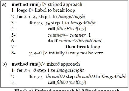
The other design given in Figure 5b can also be used with partitioned approach providing the whole image data with each thread, since neighbor pixels are needed to determine filtered pixel. However it multiplies the memory utilization by the number of parallel thread which is not practical to implement. In view of the shared approach, both design styles can be efficiently realized and threads run on the same input and output image data without splitting. On the other hand the design given in Figure 5b also eliminates the operation for determining region coordinates. Algorithms given in Figure 6a and 6b show basic implementation codes for striped and mixed methods respectively.
Fig 6: a) Striped approach b) Mixed approach
The striped approach as shown Figure 6a requires additional definitions for starting coordinates for a region and load per thread which specifies the number of pixels operations. A counter is defined to help break the operation when the thread achieved its allocated task. The mixed approach given in Figure 6b is simpler to implement. Start coordinates are determined according to thread id and are increased by the steps determined according to the number of threads. The method filterPixel() defines the convolution filtering operations according to specified filter weights. It accepts the pixel at (x,y) coordinates from the input image applies the convolution filter and returns the filtered pixel.
3.3
Implementation with Dynamic Load
Scheduling
[image:3.595.324.539.243.331.2]The efficiency of the parallel algorithm strictly depends on execution times of parallel running threads where the computational load is distributed. It is necessary for performance increase to start all threads by the same time for parallel run and that to terminate all threads by the same. However, context switches in some cores may occur during the execution of threads due to other running processes. These types of interferences usually delay the execution of some threads which in consequence delay the whole process. Figure 7 shows an illustrating example for fixed load approach using three parallel running threads with some delays. These delays cause deteriorations in the overall performance of parallel algorithm.
Fig 7: An illustration for thread delays for three parallel running threads
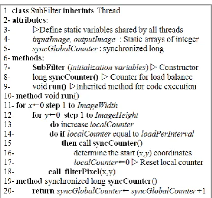
[image:3.595.54.271.439.593.2]A control mechanism can be used to utilize the faster threads to compensate thread delays by assigning more loads. For this purpose, a self-scheduling parallelism where a shared variable as a counter for organizing the loads of threads can be used during running [16,17]. According to this approach, each thread increases the counter and uses the increased value for determining the start coordinates to continue filtering. Because the counter is defined as synchronized it can only be increased by a unique thread at a time. Therefore filtering the same region more than one thread is prevented. The period of increasing the counter for task demand can be varied from one pixel to a number of pixels filtering operations. As will be discussed in the experimental results keeping the period of control tight may result in overhead as will be discussed in experimental results. Figure 8a and 8b show the example distributions of pixels for 10×10 image using three threads. Figure 8a shows the case where uniform distribution of load to cores is fully satisfied. The non - uniform distribution is illusrated in Figure 8b where a period utilizes a two core for example.
Fig 8: Example distributions for three thread executions a) uniform b) non-uniform
[image:3.595.318.544.557.654.2]These operations continue till synchronized counter reach its max value.
Fig 9: Pseudo code for dynamic load scheduling
4.
EXPERIMENTAL RESULTS
In this section, comparative experimental results to show the efficiency of presented approaches were investigated. Because, the focus of the paper is the implementation of the parallel processing algorithm on a single - chip multi - core computer for practical purposes, the experimental results were obtained a desktop computer which has a six core CPU. The model of the processor used to obtain experimental results is AMD Phenom II 1055T which has 128 KB L1 and 512KB L2 cache memory per core and 6MB L3 cache memory. The results were obtained on Windows 7 operation system where Java version 1.7.0_03. Image read/write operations in this study was realized by BufferedImage class which is included in a foundation package called java.awt.image. For higher speed, complete image is read as an array instead of calling getRGB method during filtering for reading image pixels.
4.1
Comparison of the shared and
partitioned approaches
[image:4.595.55.264.95.290.2]In this experiment performance of the parallel algorithm was evaluated in view of the two design approaches where the image is defined as shared and partitioned data types. Comparative results given by the Table 1 show that shared and partitioned approaches give the same execution times of individual threads. Because all cores access the memory using the same hardware utilities, shared approach provides a similar performance while eliminating the additional cost of dividing image data into the number of parallel threads.
Table 1. Example measurements in milliseconds (Image size: 1800 × 1800, filter size: 3 × 3)
Shared Partitioned Threads Run 1 Run 2 Run 3 Run 1 Run 2 Run 3 Thread 1 37.65 37.97 38.19 37.59 37.63 38.55 Thread 2 38.47 38.62 38.72 37.76 38.35 37.86 Thread 3 37.62 37.59 37.66 37.42 38.54 38.23 Thread 4 38.51 38.64 38.65 37.99 37.86 38.34 Thread 5 38.61 38.62 38.31 38.49 37.56 38.26 Thread 6 38.68 38.85 38.70 38.24 38.43 37.75
4.2
Comparison of the fixed load and
dynamic load scheduling approaches
The experimental results obtained above either shared or partitioned approaches use fixed load assignment to threads. However, when one or more core isn’t available due to context switches, threads may not finish their task by the same time and therefore differences in the times may occur. Because of the fork - join structure, a delay in a thread also delays the whole process. A more efficient approach for coping with duration irregularities can be implemented by using shared approach. While partitioned approach provides higher data locality, share approach takes the advantage of large L3 cache memory. For this purpose, a synchronized counter to keep track of the block operations for dynamic load scheduling can be used, as discussed previously. Because all of the threads try to access the same variable for determining filtering coordinate, frequent accesses may results in significant overheads during running. On the other hand, the overhead may be reduced by keeping the chunk sizes over some specified number of pixels operations. Before experiments for testing the effect of chunk size, the overhead time in parallel run can be measured by the Equation (2) [18].
p n T p n T p n To
) 1 , ( ) , ( ) ,
( (2)
Where T(n,p) shows execution time of a parallel algorithm, T(n,1) shows execution time for single core implementation, n is the load and p is the number of processors. In practice T(n,1) determined approximately from example runs. In order to measure the efficiency of the dynamic load scheduling approach to fixed one Equation 2 can be reorganized as in Equation 3.
) , ( ) , , ( )
, ,
(n pi T n pi T n p
To dynamic fixed (3)
Where Tdynamic(n,p,i) shows the time of dynamic algorithm, Tfixed(n,p,i) shows the time of fixed algorithm and i shows the number of pixels operations per block or in other words chunk size. Overhead measurement for dynamic algorithm relative to fixed algorithm can simply be expressed in terms of percent ratio as in Equation 4,
( , , )
% 100
( , )
o o
fixed
T n p i T
T n p
(4)
Fig 10: Experimental results for approximate To% (1200×1200 mask size 3 × 3)
Fig 11: Example threads activations during dynamic load scheduling (Image size: 1200 × 1200, filter size: 3 × 3,
chunk size: 1000 pixels)
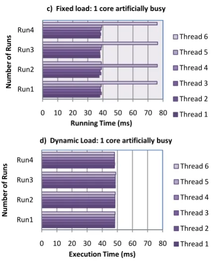
According to example consecutive runs, fixed load show serious fluctuations in the running times when compared to dynamic load scheduling. Figure 11a and 11b shows the example results for no core busy and one core busy cases respectively. While, in the first case small differences occurred in the running times, for the other cases running times are increased to about two times. The execution times obtained by dynamic load scheduling significantly low for no core busy and one core busy cases as shown in Figure 11d, 11e and 11f respectively. Therefore idle durations of the threads that finish their tasks in advance were utilized to compensate the delays in other threads by means of dynamic load scheduling approach. Figure 12 shows random execution results under variable conditions where some of the cores were made artificially almost half busy by setting about 5 ms busy and 5 ms idle actions. Figure 12a and 12b shows the execution times of the algorithm under busy conditions. According to results, considerable reductions when compared to fixed load implementation were achieved. Thread loads which show their activation in the process were presented in Figure 13. The number of pixels operation per thread is close
[image:5.595.66.277.185.503.2]to each other as shown in Figure 13a and 13b for fixed and dynamic methods respectively. For this experiment, there is no artificially busy core during running. Figure 13c and 13d show the example results where one of the cores was made artificially busy using fixed and dynamic methods respectively. The thread activations for fixed method show that one of the threads didn’t process any pixel of the image during processing. This increases the execution duration by two fold. This is eliminated in dynamic method by distributing the load during runtime.
Fig 12: Example test results for artificially busy cases (image: 1800 × 1800, filter: 3 × 3, chunk size: 1000 pixels)
0.00 5.00 10.00 15.00 20.00 25.00 30.00
25 50 100 250 500 1000
To
%
Chunk size (Number of pixels)
2 Thread 4 Thread 6 Thread 0 100000 200000 300000 400000 500000 600000 700000
Run1 Run2 Run3 Run4
P ix e ls O pe rat ions pe r Thre ad
Number of Runs a) No core artificially busy
Thread 1 Thread 2 Thread 3 Thread 4 Thread 5 Thread 6 0 100000 200000 300000 400000 500000 600000 700000
Run1 Run2 Run3 Run4
P ix e ls O pe rat ions pe r Thre ad
Number of Runs b) One core artificially busy
Thread 1 Thread 2 Thread 3 Thread 4 Thread 5 Thread 6 37 37.5 38 38.5 39 39.5 40 40.5 41
1 3 5 7 9 11 13 15 17 19
Ex e cut ion ti m e (m s)
Number of Run
a) Execution times for no core busy case
Fixed Dynamic 0 20 40 60 80 100 120
1 3 5 7 9 11 13 15 17 19
Ex e cut ion ti m e (m s)
Number of Run
b) Execution times for one core busy case (total ~17%)
Fixed
Dynamic
0 5 10 15 20 25 30 35 40 45 Run1
Run2 Run3 Run4
Running Time (ms)
Num
be
r
of
Runs
a) Fixed load: No core artificially busy
Thread 6 Thread 5 Thread 4 Thread 3 Thread 2 Thread 1
0 5 10 15 20 25 30 35 40 45 Run1
Run2 Run3 Run4
Execution Time (ms)
Num
be
r
of
Runs
b) Dynamic Load: No core artificially busy
[image:5.595.316.535.489.754.2]Fig 13: Running times for example cases. (Image size:1200×1200, filter size: 3×3, chunk size: 500 pixels)
4.3
Speed - up and parallel efficiency
In this experiment, it was shown how the number of processor affects the performance. The success of the parallel algorithm was evaluated by comparing it to single core application. Measurement of the performance is usually calculated by using “Speedup” value referring to how many times the algorithm runs faster than the sequential one [18]. Speedup is determined by dividing the execution time of the single - core application to multi - core application as given by Equation 5.( ,1) ( , )
T n Speedup =
T n p
(5)
In another criterion called “Parallel Efficiency”, the number of cores used in execution is also incorporated. It reveals the contribution of a core to the performance of parallel algorithm. It is calculated by dividing the speedup to the number of cores as given by Equation 6. The resulting value varies between 0-1 where 1 shows full efficiency of the parallel running cores.
p Speedup fficiency=
Parallel E (6)
Experimental results that measuring the speed up and parallel efficiency of the parallel image filter are given in Figure 14a and 14b respectively. Speed up versus the number of threads show good performance results. However, as the number of threads is increased, performance characteristics deviate from linearity. The same behavior was also observed in the parallel efficiency evaluations. It can also be concluded that increasing the image size has the improving effect on the parallel performance as the number of pixels operation is increased per core.
Fig 14: a) Speedup and b) Parallel efficiency results (image size: 1200 × 1200, filter size: 3 × 3, chunk size: 1000
pixels )
5.
CONCLUSIONS
Support for multithreading application in Java, enables an efficient and practical way to implement image convolution filter without additional libraries. According to experiments, the success of the shared image and partitioned image data approaches were close to each other. Shared definition of image data considerably simplifies the parallel algorithm by eliminating the splitting operations, merging and image padding of sub images. Shared approach provides the threads with the freedom of processing any pixels of the input image. This property was shown to simplify implementing a control mechanism for the dynamic load scheduling of the threads. Comparisons between fixed and dynamic load scheduling approaches showed that the irregularities in the running times of parallel threads were reduced by a simple dynamic control. Although, check intervals for load scheduling should be selected to over a certain number of pixels operations, for tested values satisfying results were observed. The results show that good speed up and parallel efficiency can be obtained practically on widely used multicore computers and Java platform.
0 10 20 30 40 50 60 70 80 Run1
Run2 Run3 Run4
Running Time (ms)
Num
be
r
of
Runs
c) Fixed load: 1 core artificially busy
Thread 6
Thread 5
Thread 4
Thread 3
Thread 2
Thread 1
0 10 20 30 40 50 60 70 80 Run1
Run2 Run3 Run4
Execution Time (ms)
Num
be
r
of
Runs
d) Dynamic Load: 1 core artificially busy
Thread 6
Thread 5
Thread 4
Thread 3
Thread 2
Thread 1
1 2 3 4 5 6
2 4 6
Speep Up
Num
be
r
of
T
hr
e
ads
(a) Speep Up versus the number of threads
2500x2500
1800x1800
1200x1200
600x600
0.8 0.85 0.9 0.95 1
2 4 6
Parallel Efficiency
Num
be
r
of
T
hr
e
ads
(b) Parallel Efficiency versus the number of threads
2500x2500
1800x1800
1200x1200
[image:6.595.323.535.74.320.2]19
6.
REFERENCES
[1] M.Kutila, J.,Viitanen, “Parallel Image Compression and Analysis with Wavelets”, International Journal of Signal Processing, Vol. 1, pp. 65–68, 2004
[2] T.Bräunl, “Tutorial in Data Parallel Image Processing”, Australian Journal of Intelligent Information Processing Systems , Vol. 6, pp. 164–174, 2001
[3] J. Kepner, “A Multi-Threaded Fast Convolver for Dynamically Parallel Image filtering”, Journal of Parallel and Distributed Computing, Vol.63, pp. 360–372,2003 [4] G. Damiand, D.Coeurjolly, “A Generic and Parallel
Algorithm for 2D Digital Curve Polygonal Approximation”, Journal of Real-Time Image Proc, Vol. 6, pp.145–157, 2011
[5] P. Frost Gorder, “Multicore Processors for Science and Engineering”, IEEE Computing in Science & Engineering, Vol.9, pp. 3-7,2007
[6] G. Andrews, Foundations of Multithreaded, Parallel, and Distributed Programming, Addison-Wesley, 2000 [7] F.Warg, P.Stenstrom, “Dual-thread Speculation: A
Simple Approach to Uncover Thread-level Parallelism on a Simultaneous Multithreaded Processor”, International Journal of Parallel Programming, Vol.36, pp.166–183,2008
[8] B. Sanden, “Coping with Java threads”, IEEE Computer, Vol. 37, pp. 20-27,2004
[9] D. Lea, Concurrent Programming in Java: Design Principles and Patterns, Addison-Wesley, 1997
[10]S. Yu, M. Clement, Q. Snell, B. Morse, “Parallel algorithms for image convolution”, Proceedings of the
International Conference on Parallel and Distributed Techniques and Applications, Las Vegas, Nevada, 1998 [11] A. S. Grimshaw, W. T. Strayer, P. Narayan, “Dynamic,
Object-Oriented Parallel Processing”, IEEE Parallel and Distributed Technology: Systems and Applications, Vol. 1, pp. 33–47,1993
[12] J. F. Karpovich, M. Judd, W. T. Strayer, A. S. Grimshaw, “A Parallel Object-Oriented Framework for Stencil Algorithms”, IEEE International Symposium on High Performance Distributed Computing, pp. 34-41,1993
[13]S.Nakariyakul, “Fast spatial averaging: an efficient algorithm for 2D mean filtering”, The Journal of Supercomputing, DOI: 10.1007/s11227-011-0638-9, Online, 2011
[14] R. C. Gonzalez, R. E. Woods, Digital Image Processing, Prentice Hall, 2008
[15]W. D. Hillis , G. L. Steele, “Data Parallel Algorithms”, Communications of the ACM, Vol.29,pp.1170-1183, 1986
[16]K. K. Yue, D. J. Lilja, “Parallel Loop Scheduling for High-Performance Computers”, High-Performance Parallel Computing Research Group Technical Report No. HPPC-94-13, 1994
[17] Z.Fang, P. Tang, P.C. Yew, C. Q. Zhu, “Dynamic processor self-scheduling for general parallel nested loops”, Vol. 39, pp. 919 – 929,1990
[18]Z. Juhasz, “An Analytical Method for Predicting the Performance of Parallel Image Processing Operations”,
The Journal of Supercomputing,