Application of Speech Signals to Deterministic
Signal Modeling Techniques
D.Vijaya Lakshmi
M.Tech (RADAR &Microwave Engineering), Assistant Professor, Department of E.C.E,
AN.I.T.S, Visakhapatnam.
G.Gayatri
M.Tech (RADAR &Microwave Engineering), Assistant Professor, Department of E.C.E.,
A.N.I.T.S., Visakhapatnam
ABSTRACT
Signal modeling is concerned with the representation of signals. The modeled signal consists of parameters, using which the original signal can be reconstructed or recovered. When once it is possible to accurately model a signal, then it becomes possible to perform important signal processing tasks such as signal compression, interpolation, prediction. The models used are AR (Auto Regressive) or All-Pole model, MA (Moving Average) or All-Zero model, ARMA (Auto Regressive Moving Average) or Pole-Zero model. Various methods have been suggested for the coefficients determination among which are Prony, Pade, Shank, Autocorrelation, Covariance techniques.
In this paper, these techniques are applied for speech signals and comparisons are carried out. The comparisons are entirely based on the value of the coefficients obtained.
Keywords
Pade, Prony, Shank, Auto Regressive, Moving Average, Autoregressive Moving Average.
1.
INTRODUCTION
The use of modeling technique to predict or reconstruct a data sequence is concerned with the representation of data in an efficient technique [1]. Signal modeling have been used in radar application, geophysical application, Medical signal processing, ultrasonic tissue backscatter coefficient estimation, speech processing, music understanding and more recently in the field of Magnetic Resonance Imaging (MRI) reconstruction [7].
Signal modeling involves two steps [1], these are;
1) Model selection: Choosing an appropriate parametric form for the model data
2) Model Parameter determination: This includes model order and model coefficients determination.
Despite the success reported in the use of modeling technique, two important problems constitutes challenges to the applicability of this method, these are:
1) Estimation of Model order: There has been various efforts in determining a workable criteria for the determination of an appropriate model order. The use of a model with an order too high over fits the data while the use of a model with a low order leads to insensitivity to noise [1].
2) Estimation of model coefficient: The second important challenges mitigating against the use of modeling technique is the estimation of the model coefficients. Some of the existing methods of determining model coefficients include Prony,
Pade, Least Square, Shank, Autocorrelation, Autocovariance methods [1].
2.
SIGNAL MODELING TYPES
A linear system's transfer function
H
(
z
)
is given by
pk
k p q k
k q p
q
z
k
a
z
k
b
z
A
z
B
z
H
1 0
)
(
1
)
(
)
(
)
(
)
(
(1)Different models related to deterministic signals have three specific models [4]:
1. Auto Regressive (AR) Process. 2. Moving Average (MA) Process.
3. Auto Regressive Moving Average (ARMA) Process.
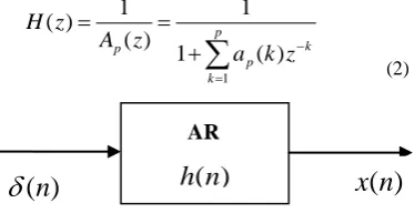
Auto Regressive (AR) Process:
In this case, only poles will be present i.e. the linear filter
H
(
z
)
1
A
p(
z
)
. Hence, thisprocess is also called asan all pole filter. The system function of AP process is given by,
(2)
[image:1.595.332.519.474.570.2]
Figure. 1: Block Diagram of AR Process. Mathematical Modeling of AR Process:
From Figure. 1, the output
x
(
n
)
is the convolution of the input signal
(
n
)
and the system function of the filterh
(
n
)
i.e.1
)
(
1
)
(
1
)
(
)
(
)
(
1
)
(
1
)
(
)
(
)
(
)
(
1
p
k
k p p
p
z
k
a
z
X
z
A
z
X
z
A
z
H
z
X
n
h
n
n
x
)
(
n
h
)
(
n
x
(
n
)
AR
pk
k p
p
z
a
k
z
A
z
H
1
)
(
1
1
)
)
(
n
h
)
(
n
x
y
(
n
)
MA
p k p p k p p k pk
n
x
k
a
n
n
x
n
k
n
x
k
a
n
n
x
n
k
n
x
k
a
n
x
1 1 1)
(
)
(
)
(
)
(
)
(
)
(
)
(
)
(
)
(
)
(
)
(
)
(
)
(
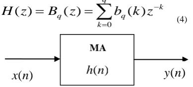
Moving Average (MA) Process:
In this case, only zeros will be present i.e. the linear filter
H
(
z
)
B
q(
z
)
. Hence, thisprocess is also called as allzero filter[4]. The system function of MA process is given by
[image:2.595.311.549.211.586.2](4)
Figure. 2: Block Diagram of MA Process. Mathematical Modeling of MA Process:
From Figure. 2, the output
y
(
n
)
is the convolution of the inputx
(
n
)
and the system function of the filterh
(
n
)
i.e.
q k q q kk
n
x
k
b
n
y
k
n
x
k
h
n
y
n
h
n
x
n
y
0 0)
(
)
(
)
(
)
(
)
(
)
(
)
(
)
(
)
(
Auto Regressive Moving Average Process:
In this case, both poles and zeros will be present i.e. the linear
filter
)
(
)
(
)
(
z
A
z
B
z
H
p q
. Hence, thisprocess is also called aspole zero filter[4]. The system function of ARMA process is given by
p k k p q k k q p qz
k
a
z
k
b
z
A
z
B
z
H
1 0)
(
1
)
(
)
(
)
(
)
(
(6)Figure. 3: Block Diagram of ARMA Process.
Mathematical Modeling of ARMA Process:
From Figure. 3, the output
x
(
n
)
is the convolution of the input
(
n
)
and the system function of the first filter)
(
1n
h
i.e.
p kp
k
x
n
k
a
n
n
x
1)
(
)
(
)
(
)
(
(7)where the system function is given by,
)
(
1
)
(
1
z
A
z
H
p
(8)The output
y
(
n
)
is the convolution of the inputx
(
n
)
and the system function of the second filterh
2(
n
)
i.e.)
(
)
(
)
(
n
x
n
h
2n
y
qk
q
k
x
n
k
b
n
y
0)
(
)
(
)
(
q k p p pq
k
n
k
a
k
g
n
k
b
n
y
0 1)
2
(
)
(
)
(
)
(
)
(
)
(
)
2
(
)
(
)
(
)
(
)
(
0 0 1
k
b
k
n
x
k
a
k
n
k
b
n
y
q q k q k p k pq
(9)3.
MODELING PROCEDURE
The goal of signal modeling is to produce a signal which should be as close as possible to with input to the filter as impulse signal [1].
Figure. 4: Modeling Procedure
Any deterministic signal can be generated by linear time invariant filter driven with unit impulse function
(
n
)
[6]. This is shown in Figure. 4.The steps followed for modeling a signal are: 1. Generation of analog signal. 2. Discretization of the signal.
3. In this step
H
(
z
)
is found out using different method.4. H(z)is driven with
(
n
)
then the signal obtained approximate the signal)
(
1
)
(
z
A
z
H
AR
p
)
(
)
(
z
B
z
H
MA
q) ( ) ( ) ( z A z B z H ARMA p q
)
(
n
)
(
)
(
ˆ
n
x
n
x
)
(
n
x
q k k qq
z
b
k
z
B
z
H
0)
(
)
(
)
(
) (n x(3)
(5))
(
ˆ
n
x
(9)
)
(
n
x
(
n
)
y
(
n
)
[image:2.595.63.258.241.329.2])
(
ˆ
n
b
)
(
n
x
e
(
n
)
)
(
n
b
q-
+
) ( ) ( ) ( z A z B z H p q 4.
METHODS OF COEFFICIENTS
DETERMINATION
Various methods have been reported in literatures for determining the AR/ARMA model coefficients, among which are [4]:
4.1
Direct least square method
The block diagram for direct method of least square solution is as shown in Figure. 1 the modeling error can be written as e(n) = x(n) − h(n)
2 0
)
(
'
nLS
e
n
(10) A necessary condition for the filter coefficients to minimize the squared error is to calculate the partial derivative of
LSwith respect to each of the coefficients
a
p(
k
)
&
b
q(
k
)
vanish, i.e.0
)
(
k
a
p LS
;k
1
,
2
,
p
(11)
0
)
(
k
b
q LS
;k
1
,
2
,
q
(12)Using Parseval’s theorem, the least squares error may be written in frequency domain as
d
e
E
j LS
2)
(
2
1
To find the denominator coefficients
a
p(
k
),
set the partial derivative of
LS with respect toa
p(
k
)
equal to zero
(
)
(
)
0
2
1
)
(
'
d
e
E
e
E
a
k
a
j j p p LS (13) Since,)
(
)
(
)
(
)
(
j p j q j je
A
e
B
e
X
e
E
(14) On substitution of Eq. (14), the Eq. (13) becomes
0
)
(
*
)
(
*
)
(
)
(
2
1
)
(
*
2
d
e
e
A
e
B
e
A
e
B
e
X
k
a
jk j p j q j p j q j p LS (15) fork
1
,
2
,
p
Similarly, to find the numerator coefficients set the partial
derivative of
LS with respect tob
q(
k
)
equal to zero
(
)
(
)
0
)
(
2
1
)
(
d
e
E
e
E
k
b
k
b
j j q q LS (16) Since,)
(
)
(
)
(
)
(
j p j q j je
A
e
B
e
X
e
E
(17) On substitution of Eq. (17), the Eq. (16) becomes
0 ) ( * ) ( ) ( ) ( 2 1 ) ( *
d e A e e A e B e X k b j p k j j p j q j q LS (18) fork
1
,
2
,
q
But, it is clear that from the Eq. (15) and (18) that the optimum set of model parameters are defined implicitly in terms of a set of p+q+1 nonlinear equations.
Limitation
The limitation with least squares method is that the equations results to a set of non-linear equations. Therefore, this approach is not mathematically tractable and not amenable in real-time signal processing applications.
4.2
Pade Approximation
The development of Pade method begins by expressing the system function as [3],
p k k p q k k q p q z k a z k b z A z B z H 1 0 ) ( ) ( ) ( ) ( ) (which leads to the difference equation
p k n q b k n h k p a n h 1 ) ( ) ( ) ( ) ( (19) To find the coefficients ap(k) &b
q(
k
)
that give an exact fitof the data to model over the interval [0, p+q], equate
) (n
h and x(n) then the Eq. (19) changes to
p k q pn
b
k
n
x
k
a
n
x
10
)
(
)
(
)
(
)
(
(20) Limitation There isno guarantee on how accurate the model will be for values of n outside the interval [0, p+q]. In some cases, the match may be very good, while in others it may be poor.
4.3
Prony method
The block diagram of Prony’s method of signal modeling is shown in Figure. 5 [1]. The modeling error defined as the difference between the input and the output of the filter is given by
)
(
)
(
)
(
'
n
x
n
h
n
e
(21)) ( ) ( ) ( ) ( ) ( ) ( z A z B z X z H z X z E p q
Figure: 5: System interpretation of Prony’s method for signal modeling.
Multiplying both sides of Eq. (21) with a new error is obtained as
)
(
)
(
)
(
)
(
)
(
)
(
z
A
z
E
z
A
z
X
z
B
z
E
p
p
q(22) ; n = 0, 1 …q
;
n = q
+ 1,
q
+2…
p+q
;
n =
0, 1 …q
; n = q+ 1, q+2… p+q
; for
10
)
(
)
(
q nk
n
x
n
e
; fork
1
,
2
,
p
) ( 1 z Ap
)
(
n
g
(
n
)
e
(
n
)
)
(
n
x
)
(
ˆ
n
x
+
-
and in time-domain Eq. (22) is given by
)
(
)
(
ˆ
)
(
)
(
)
(
)
(
n
a
n
x
n
b
n
b
n
b
n
e
p
q
q
q(23)
where
(
)
(
)
(
)
ˆ
n
a
n
x
n
b
q
p
Since
b
q(
n
)
0
for n>q, the error is expressed as, (24)
1 2 ,(
)
q n qp
e
n
(25)
setting the partial derivatives of
p,qwith respect to a *(k)p
equal to zero [3], gives
1 ,)
(
*
)
(
*
)
(
)
(
*
n q pp q p
k
a
n
e
n
e
k
a
0
)
(
)
(
)
(
)
(
)
(
)
(
1 1
q n p k p pp
a
k
k
n
x
l
a
n
a
n
x
n
e
(26)Since the partial derivative of e*(n) with respect to
)
(
*
k
a
p isx
*
(
n
k
)
Eq. (3.31) becomesSubstitute Eq. (24) for
e
(
n
)
into Eq. (26),0 ) ( ) ( ) ( ) ( 1 1
xn
a l xn l x n kq n p l p or equivalently,
1 1) ( ) ( ) ( q n p l
p l xn l x n k
a =
1 ) ( ) ( q n k n x n x
p k x xp k r k l r k
a 1 ) 0 , ( ) , ( ) (
p
k
1
,
2
,
(27)where
1)
(
)
(
)
,
(
q nx
k
l
x
n
l
x
n
k
r
4.4
Shank method (Modified Prony)
[image:4.595.56.281.69.585.2]Shank method is a modified Prony method in the sense that the moving average coefficients is obtained by finding the least square minimization of the model error over the entire data length [4]. The model can be viewed as a cascade of two filters, Bq(z) andAp(z).
Figure. 6: System interpretation of Shank’s method for signal modeling.
The cascade of two filters
A
p(
z
)
andB
q(
z
)
are shown in the Fig.6 and its system function is given by ) ( 1 ) ( ) ( z A z B z H p
q (28)
From Figure. 6, the unit sample response g(n) of the first filter
1
A
(
z
)
p is determined with
g
(
n
)
0
forn
0
i.e.)
(
)
(
)
(
n
n
a
n
g
p
i.e
p
k
p k g n k
a n n g 1 ) ( ) ( ) ( ) (
(29) The minimum squared error is defined as2 0
)
(
ns
e
n
minimizing the error in Prony method gives
q l xg gq l r k l r k
b 0 ) ( ) ( )
( ;
k
0
,
1
,
q
(30)
0)
(
*
)
(
)
,
(
)
(
n gg
k
l
r
k
l
g
n
l
g
n
k
r
and
0)
(
*
)
(
)
(
nxg
k
x
n
g
n
k
r
5.
APPLICATION OF SIGNAL
[image:4.595.315.524.453.492.2]MODELING TO SPEECH SIGNALS
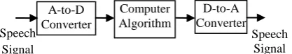
Speech coding or speech compression is the field concerned with obtaining compact digital representations of speech signals for the purpose of efficient transmission or storage. The aim in speech coding is to represent speech by a minimum number of bits while maintaining its perceptual quality[2].Figure. 7: General block diagram for application of digital signal processing to speech signals
.
The block diagram in Figure. 7 represents any system where time signals such as speech are processed by the techniques of DSP. This figure simply depicts the notion that once the speech signal is sampled, it can be manipulated in virtually limitless ways by DSP techniques.
5.1
Basic Procedure of Signal Modeling
Any deterministic signal can be generated by linear time-invariant filter driven with impulse function. The procedure of signal modeling to be followed when applied to speech signals are as follows:
1. Discretization of analog speech signal.
2. Application of modeling methods to the speech signal (model parameters are obtained).
3. The transfer function of the filter H(z)is driven with impulse signal
(n), and then the original speech signal is obtained.; n = 0, 1, q
; n > q
6.
SIMULATION & RESULTS
Application of Speech Signals to Signal Modeling Methods Pade, Prony’s and Shank’s methods of signal modeling are realized for AR, MA, and ARMA models. For each of these models the inputs are
: ) (n
x The speech signal to be modeled, p :Number of poles and
q :Number of zeros.
(Here the number of poles and zeros represent the order of the model).
and the outputs are
a : The filter coefficients representing the denominator part of the system function
b : The filter coefficients representing the numerator part of the system function and
)
(
n
e
: Error in the estimated signal.An error is generated if p+q > = length of
x
(
n
)
. So, the values of p and q must be selected such that their sum is less than the length ofx
(
n
)
.6.1
Pade Approximation Method
First, the speech signal which is in the continuous or analog form is considered. Then the numerator and denominator coefficients are calculated by applying the discrete speech signal to Pade approximation method algorithm. Applying the impulse signal as the input to the filter and using these coefficients, the output signal of the filter
y
(
n
)
is obtained. The error signal is calculated as the difference between the input signalx
(
n
)
and output signal y(n). In order to get the signal y(n) as close as possible to the signalx
(
n
)
, the number of poles and zeros in the algorithm have to be varied.6.1.1
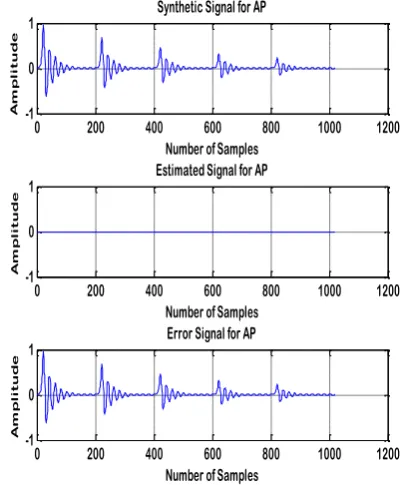
AP Model
The input is considered to be a speech signal with filename speech_10k. The number of poles is considered to be
205
p
. The Figure. 8 shows the original, estimated (or reconstructed) speech signals and the error obtained.6.1.2
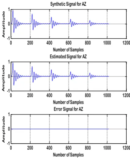
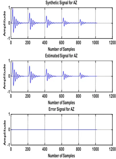
AZ Model
The input is considered to be a speech signal with filename speech_10k. The number of zeros is considered to be
1018
q . The Figure. 9 shows the original, estimated (or reconstructed) speech signals and the error obtained.
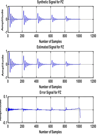
6.1.3
PZ Model
The input is considered to be a speech signal with filename speech_10k. The number of poles and zeros are considered to be p200 and q140. The Figure. 10 shows the original, estimated (or reconstructed) speech signals and the error obtained.
0 200 400 600 800 1000 1200
-1 0 1
Number of Samples
A
m
p
li
t
u
d
e
Synthetic Signal for AP
0 200 400 600 800 1000 1200
-2 0 2x 10
-4
Number of Samples
A
m
p
li
t
u
d
e
Estimated Signal for AP
0 200 400 600 800 1000 1200
-1 0 1
Number of Samples
A
m
p
li
t
u
d
e
[image:5.595.329.539.88.328.2]Error Signal for AP
Figure. 8: Signal modeling using Pade Approximation method for AP model.
0 200 400 600 800 1000 1200
-1 0 1
Number of Samples
A
m
p
li
t
u
d
e
Synthetic Signal for AZ
0 200 400 600 800 1000 1200
-1 0 1
Number of Samples
A
m
p
li
t
u
d
e
Estimated Signal for AZ
0 200 400 600 800 1000 1200
-1 0 1
Number of Samples
A
m
p
li
t
u
d
e
Error Signal for AZ
[image:5.595.329.542.376.634.2]0 200 400 600 800 1000 1200 -1
0 1
Number of Samples
A
m
p
li
t
u
d
e
Synthetic Signal for PZ
0 200 400 600 800 1000 1200 -1
0 1
Number of Samples
A
m
p
li
t
u
d
e
Estimated Signal for PZ
0 200 400 600 800 1000 1200 -0.2
0 0.2
Number of Samples
A
m
p
li
t
u
d
e
[image:6.595.67.290.82.347.2]Error Signal for PZ
Figure. 10: Signal modeling using Pade Approximation method for PZ model.
6.2
Prony’s Method
First, the speech signal which is in the continuous or analog form is considered. Then the numerator and denominator coefficients are calculated by applying the speech signal to Prony’s method algorithm. Applying the impulse signal as the input to the filter and using these coefficients, the output signal of the filter
y
(
n
)
is obtained. The error signal is calculated as the difference between the input signalx
(
n
)
and output signal
y
(
n
)
. In order to get the signaly
(
n
)
as close as possible to the signalx
(
n
)
, the number of poles and zeros in the algorithm have to be varied.6.2.1
AP Model
The input is considered to be a speech signal with filename speech_10k. The number of poles is considered to be
p
1
. Figure.11 shows the original, estimated (or reconstructed) speech signals and the error obtained.6.2.2
AZ Model
The input is considered to be a speech signal with filename speech_10k. The number of zeros is considered to be
q
1018
. Figure.12 shows the original, estimated (or reconstructed) speech signals and the error obtained.6.2.3
PZ Model
The input is considered to be a speech signal with filename speech_10k. The number of poles and zeros are considered to be
p
198
andq
209
. Figure.13 shows the original, estimated (or reconstructed) speech signals and the error obtained.0 200 400 600 800 1000 1200
-1 0 1
Number of Samples
A
m
p
li
t
u
d
e
Synthetic Signal for AP
0 200 400 600 800 1000 1200
-1 0 1
Number of Samples
A
m
p
li
t
u
d
e
Estimated Signal for AP
0 200 400 600 800 1000 1200
-1 0 1
Number of Samples
A
m
p
li
t
u
d
e
[image:6.595.326.527.86.329.2]Error Signal for AP
Figure. 11: Signal modeling using Prony’s method for AP model.
0
200
400
600
800
1000
1200
-1
0
1
Number of Samples
A
m
p
l
i
t
u
d
e
Synthetic Signal for AZ
0
200
400
600
800
1000
1200
-1
0
1
Number of Samples
A
m
p
l
i
t
u
d
e
Estimated Signal for AZ
0
200
400
600
800
1000
1200
-1
0
1
Number of Samples
A
m
p
l
i
t
u
d
e
[image:6.595.327.531.380.694.2]Error Signal for AZ
0 200 400 600 800 1000 1200 -1
0 1
Number of Samples
A
m
p
li
t
u
d
e
Synthetic Signal for PZ
0 200 400 600 800 1000 1200 -1
0 1
Number of Samples
A
m
p
li
t
u
d
e
Estimated Signal for PZ
0 200 400 600 800 1000 1200 -0.1
0 0.1
Number of Samples
A
m
p
li
t
u
d
e
[image:7.595.68.282.84.366.2]Error Signal for PZ
Figure. 13: Signal modeling using Prony’s method for PZ model.
6.3
Shank’s Method
First, the speech signal which is in the continuous or analog form is considered. Then the numerator and denominator coefficients are calculated by applying the speech signal to Shank’s method algorithm. Applying the impulse signal as the input to the filter and using these coefficients, the output signal of the filter
y
(
n
)
is obtained. The error signal is calculated as the difference between the input signalx
(
n
)
and output signal
y
(
n
)
. In order to get the signaly
(
n
)
as close as possible to the signalx
(
n
)
, the number of poles and zeros in the algorithm have to be varied.6.3.1
AP Model
The input is considered to be a speech signal with filename speech_10k. The number of poles is considered to be
205
p . Figure.14 shows the original, estimated (or reconstructed) speech signals and the error obtained.
6.3.2
AZ Model
The input is considered to be a speech signal with filename speech_10k. The number of zeros is considered to be
z
1018
. Figure.15 shows the original, estimated (or reconstructed) speech signals and the error obtained.0 200 400 600 800 1000 1200 -1
0 1
Number of Samples
A
m
p
li
t
u
d
e
Synthetic Signal for AP
0 200 400 600 800 1000 1200 -0.2
0 0.2
Number of Samples
A
m
p
li
t
u
d
e
Estimated Signal for AP
0 200 400 600 800 1000 1200 -1
0 1
Number of Samples
A
m
p
li
t
u
d
e
Error Signal for AP
Figure. 14: Signal modeling using Shank’s method for AP model.
0 200 400 600 800 1000 1200 -1
0 1
Number of Samples
A
m
p
li
t
u
d
e
Synthetic Signal for AZ
0 200 400 600 800 1000 1200 -1
0 1
Number of Samples
A
m
p
li
t
u
d
e
Estimated Signal for AZ
0 200 400 600 800 1000 1200 -1
0 1
Number of Samples
A
m
p
li
t
u
d
e
[image:7.595.325.533.91.370.2]Error Signal for AZ
[image:7.595.333.537.418.697.2]6.3.3
PZ Model:
The input is considered to be a speech signal with filename speech_10k. The number of poles and zeros are considered to be
p
200
andz
220
.Figure. 16 shows the original, estimated (or reconstructed) speech signals and the error obtained.0 200 400 600 800 1000 1200
-1 0 1
Number of Samples
A
m
p
li
t
u
d
e
Synthetic Signal for PZ
0 200 400 600 800 1000 1200
-1 0 1
Number of Samples
A
m
p
li
t
u
d
e
Estimated Signal for PZ
0 200 400 600 800 1000 1200
-0.1 0 0.1
Number of Samples
A
m
p
li
t
u
d
e
Error Signal for PZ
Fi gure. 16: Signal modeling using Shank’s method for PZ
model.
The Table. 1 shows the simulated results of deterministic speech signals when applied to different methods of signal modeling. From the tabulated results, we can observe that Shank’s method of signal modeling produces accurate reconstructed signal i.e. error produced is minimum.
Method Error
AP Model
Error AZ Model
Error PZ Model
Pade
Approximation Method
16.9985 0.009 0.0399
Prony’s Method 17.0006 0.005 0.0351
[image:8.595.68.259.156.417.2]Shank’s Method 16.6528 0.003 0.0260
Table. 1: Simulated Results of signal modeling methods when applied to speech signals.
7.
CONCLUSION
The project work has commenced with the development of different methods of signal modeling. The Least Squares method requires solving a set of non linear equations; therefore it is not mathematically tractable and not amenable to real time signal processing. So, here some indirect methods of signal modeling like Pade approximation, Prony’s and Shank’s methods have been developed. The Pade approximation method will always produce an exact fit to the data for the input values equal to the sum of poles and zeros. But, the limitation of this method is that there is no guarantee on how accurate the model will be for the values outside the interval. This limitation is overcome in Prony’s method, which matches the signal exactly for the input values equal to zeros of the system. Shank’s method is a modification to Prony’s method in finding the zeros of the system.
The speech signals are implemented using deterministic signal modeling methods. The purpose of all these methods is to find the model parameters and again reconstruct the original signal using those parameters. The simulated results proved that the Shank’s method has the ability to estimate accurately as compared to other methods.
All the algorithms have been implemented in MATLAB, a language of technical computing, widely used in Research, Engineering and Scientific computations.
8.
REFERENCES
[1] Monson H. Hayes, “Statistical Digital Signal Processing and Modeling” , John Wiley & Sons, INC.
[2] Thomas F. Quatieri “Discrete Time Speech Signal Processing”, Prentice-Hall, INC.
[3] Sanjit. K. Mitra, “Digital Signal Processing”, Mc Graw-Hill Companies, INC,2006 New York.
[4] Dimitris G. Manolakis, “Digital Signal Processing principles, Algorithms and Applications”, PHI.
[5] Peyton Z. Peebles, “Probability, Random Variables and Random Signal Principles”, McGraw-Hill, INC.
[6] John G. Proakis, Dimitris G. Manolakis, “Digital Signal Processing Principles, Algorithms and Applications”, PHI.
[image:8.595.49.281.536.696.2]