Design and Implementation of PID Controller with Lead
Compensator for Thermal Process
Sreeraj P V
PG Scholar Department of E&I Karunya University
ABSTRACT
PID controller is a conventional controller which uses the advantages of Proportional, derivative and Integral controllers for achieving satisfactory results. PID controller gives better results in the system response, like less overshoot, reduced settling time, less steady state error etc even for nonlinear processes, when perfectly tuned. To achieve more stability for the system, a lead compensator can also be added. Stability Boundary Locus method, a graphical method, is used for tuning the controller parameters, Kp, Ki and Kd. This technique includes less mathematical calculations. The stability of the system can be analyzed very easily with the Stability Boundary plot and Bode Plot analysis.
General Terms
Controller Tuning, PID Controller, Compensator, Stability Analysis.
Keywords
Controller Tuning, Lead compensator, PID controller, Stability boundary locus, Stability regions.
1.
INTRODUCTION
Control engineering is an engineering discipline that applies control theory to design systems with desired behaviors. It is used for analysis and design of closed loop systems, such as systems that controls temperature, flow, voltage and pressure. Control theory can be used in every phase of the process design cycle and it can be used to help engineers to understand the performance and problems, and thus to provide solutions [2].
To obtain the desired behavior, a controller senses the output of the system, calculates the error by comparing it with the desired output and thus identifies the corrective actions based on the given specifications, and actuates the system to obtain the desired changes [3]. So, in order to identify the dynamics of the system, we need a model of the system, analyzing tools, controller tuning methods, and techniques to implement them. Integrals and Derivatives are the commonly using tools for modeling a system.
In industrial process control applications, phase-lead/lag compensators are widely used next only to PID controllers [1, 2, 3]. Such controllers are tuned usually with specifications on gain and phase margins which can lead to good performance and robustness. Now for tuning the phase lead/lag compensators, specific knowledge about the frequency response of the plant is required. Such points are specified by their frequency, gain and phase and cannot be easily found out without the help of an accurate model of the plant. To the best knowledge, there is no method available to achieve gain and phase margins exactly [4]. Note also that phase lead compensators have some parameters in the denominator of its transfer function, unlike PID controllers where all the
parameters appear linearly, Thus, effective techniques for PID controllers with exact gain and phase margin specifications are not applicable to phase-lead compensators. The traditional tuning method for phase-lead/lag compensator parameters is based on the trial and error method. To attain the desired gain and phase margins, we use phase lead compensator with the PID controller.
2.
PID CONTROLLER
Proportional–Integral–Derivative (PID) controller is a generic control loop feedback mechanism (controller) widely used in industrial control systems – a PID is the most commonly used feedback controller [3]. PID controller calculates error value as the difference between a measured process variable and a set point. By adjusting the controller parameters and thus adjusting the control inputs to the process, the controller tries to minimize the error.
The PID controller calculation involves three parameters namely, proportional, integral and derivative values, denoted by P, I, and D and is often called as three-term control. In terms of time, these values can be interpreted as: P term is dependent on the current error, I as the accumulation of previous error values, and D as a prediction of future errors, based on current rate of change. The sum of these three actions is used to adjust the process via a control element. With the help of tuning algorithms, the three parameters of PID controller can be designed to meet the desired process specifications. The response of the controller can be described in terms of how fast the controller responds to an error. Note that the use of the PID algorithm for control does not guarantee optimal control of the system or system stability. (1) It is found that by introducing a lead, we could achieve more satisfactory control action and the stability of the system can be increased [13]. Also, we can develop systems that satisfy the controlled system specifications.
3.
SYSTEM IDENTIFICATION
3.1
Step Test
tool box for obtaining the transfer function model of the system.
In this work the second method is used. Given below are the steps in calculating the process model. Here the transfer function model is obtained from the step response. The steps to be followed for finding out the time constant and the process gain are as follows.
1) Note down the Initial Steady State (I.S.S) value of the process variable (PV).
2) Give a noticeable change in the input.
3) Observe the change in the process variable and note down the New Steady State (N.S.S) value. 4) Find out the total change in PV that has occurred
(2)
5) Compute the value 6) Note down the time when the process passes
through the value. Let it be .
7) Subtract from it the time when the PV starts a clear response for a change in the input signal. Let it be
8) Then the time constant (T) can be calculated as
(3)
9) The process gain will be the , where ∆V is the change in the input in Volts
10) The Delay Time will be .
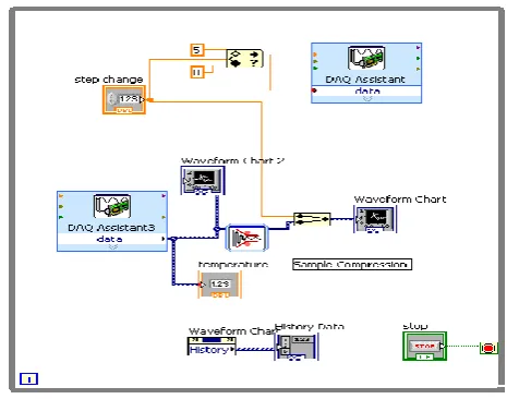
For the temperature process considered in this paper the entire process can be divided into four operating regions, i.e. the total operating region from room temperature to 100˚C can be divided into four. Figure 1 shows the LabVIEW block diagram for open loop test. An input voltage within the 0- 5 V is given as the input. In the Figure 1 step change indicates the input and the output value of the process variable are read from the DAQ. The DAQ used here is a PCI-6251.
Table 1 shows the experimental result for the step test which includes the time constant, delay time and the process gain.
From the experimental results it is clear that the process is non linear for the system characteristics keeps on changing with time. The transfer function for the two regions has been found out.
The transfer function modeling for the given temperature system is done. The transfer function is given by
(4)
[image:2.595.318.551.75.258.2]Then the next step is to tune the controller to find out the appropriate controller settings.
Figure 1: LabVIEW Block Diagram for Step Test
Table 1. Experimental Data Input
Change (V)
(∆PV*.632) +I.S.S
Process Gain (˚C/V)
Time constant
(sec)
Dead Time (sec)
0-1 30.792 6 432 22
1-2 38.32 10 249 10
4.
CONTROLLER DESIGN
4.1
Stability Boundary Locus
There has been a great amount of research work on the tuning of PI, PID controllers, since these types of controllers have been widely used in industries for several decades. Stability Boundary Locus method is one of the simplest method that can be used for tuning the parameters of PI, PID controllers [5]. In this method we need to plot the Stability Boundary Locus in the (Kp-Ki) plane. From that locus we need to describe the stability range of the Kp, Ki values.
4.1.1
Step by Step Procedure
First of all, consider a single input single output system as shown in Figure 2. [5-7]
Figure 2: A SISO control system
• Decompose the numerator and the denominator polynomials of G(jω) into their even and odd parts, and substitute s=jω
• Find out the closed loop characteristic polynomial of the system and equate to Zero
• Solve for Kp and Ki
Consider a unity feedback process with transfer function
(5)
And controller,
(6)
Decomposing the numerator and denominator into their odd
and even parts and substituting s= jω, we will get,
(7)
The CL characteristic equation can be written as,
(8)
Then equating the real and imaginary parts to zero,
(9)
(10) )
(11)
Now the equations (10) and (11) can be written as,
(12)
From the above equation,
(13)
Solving these two equations simultaneously and substituting the values for ω, the stability boundary locus, l(Kp,Ki,w), in the (Kp-Ki)-plane can be obtained. For PID controller Kp, Ki equations will have terms that contains Kd value.
We know that equation for PID controller is as given by (1),
Using the same procedure discussed above, the equations for Kp and Ki in terms of Kd can be obtained and is given in equation 14.
Assume Kd=1 in equation 14, and vary the ω value to get different Kp and Ki values.
(14)
The range of ω value can be calculated by equating the imaginary part of the transfer function to zero.
(15)
Substituting the values of and plotting the graph between Kp and Ki, the Stability Boundary locus can be found out. From this graph the parameter Tuning can be done.
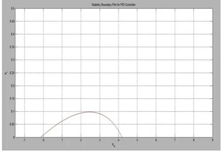
The stability boundary locus divides the parameter plane (Kp -Ki plane) into stable and unstable regions. By choosing a test point within each region, the values of stabilizing Kp and Ki parameters can be determined.
[image:3.595.315.543.340.497.2]Assume the gain margin and phase margin, according to which one will get the desired controller parameters Kp and Ki values from graph.
Figure 3: Stability Boundary Locus for PID Controller
Substituting the values of and plotting the graph between Kp and Ki, the Stability Boundary locus can be found out. From this graph the parameter Tuning can be done.
The stability boundary locus divides the parameter plane (Kp -Ki plane) into stable and unstable regions, as shown in Fig 3. By choosing a test point within each region, the stable region which contains the values of stabilizing Kp and Ki parameters can be determined [8].
Assume the gain margin and phase margin, according to which one will get the desired controller parameters Kp and Ki values from graph.
4.2
Advantages of Stability Boundary
Locus Plots
It can easily be obtained by equating the real and the imaginary parts of the characteristic equation to zero It does not require linear programming to solve a set
of inequalities
5.
LEAD COMPENSATOR
The purpose of phase lead compensator design in the frequency domain generally is to satisfy specifications on steady-state accuracy and phase margin. The specifications can also be on gain crossover frequency or closed-loop bandwidth. Phase margin specification represents the requirement on relative stability due to time delay in the system, or a representation of desired transient response characteristics that have been translated from the time domain into the frequency domain.
The overall philosophy in the design procedure presented here is for the compensator to adjust the system’s Bode phase curve to establish the required phase margin at the current gain-crossover frequency, without changing the system’s magnitude curve at that particular frequency and without reducing the zero-frequency magnitude value [8, 9]. The change or shift in the gain crossover frequency is a function of the amount of phase shift that must be added to satisfy the required phase margin. For the phase lead compensation to work, the necessary characteristics needed are given below.
The Bode magnitude curve (after the steady-state accuracy specification has been satisfied) must pass through 0 db in some acceptable frequency range; The phase shift without compensation, at the gain
crossover frequency must be more negative than the value needed to satisfy the phase margin specification (otherwise, no compensation is needed).
If the compensation is to be performed by a single-stage compensator, the degree up to which the phase curve needs to be shifted up, must be less than 90◦, at the particular gain crossover frequency and is generally restricted to a maximum value in the range 55◦–65◦. Multiple stages of compensation can be used, following the procedure explained below, and is needed when the degree that the Bode phase curve must be moved up exceeds the available phase shift for a single stage of compensation.
5.1
Design of Lead Compensator
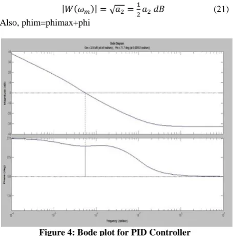
The design procedure presented here is basically graphical method. All the parameters needed, can be obtained from the Bode plot of the uncompensated system figure 4 [9]. If data arrays representing the magnitudes and phases of the system at various frequencies are available, then this design can be done numerically [13]. From the table 2, it is clear that the phase margin for the system is now 620. Now to make it 750, which corresponds to the gain value a2=4.
Now the transfer function for lead compensator can be expressed as,
(16) Upper cut off frequency,
(17)
Lower cut off frequency,
(18)
Maximum Phase shift,
(19) At frequency,
(20)
And gain at that frequency is,
[image:4.595.316.544.71.302.2](21) Also, phim=phimax+phi
Figure 4: Bode plot for PID Controller
Using these equations construct the table 2 and then substitute the apt value for a2 in equation 19
Thus, the transfer function can be derived and is found to be,
(22)
Table 2. Bode Plot Data
a2
phimax
Mag dB
ω Rad/s
Phi (Deg)
Phim (Deg)
Angle (Deg)
0
0.35 62 -118
2 3.010 19.47 -3 0.05 53 72.4 -127
3 4.771 30 -4.5 0.06 47 77 -133
4 6.020 36.86 -6.1 0.07 39 75.8 -141
5 6.989 41.81 -6.9 0.08 36 77.8 -144
6 7.781 45.58 -7.7 0.09 28 73.5 -152
7 8.451 48.59 -8.5 0.09 25 73.5 -155
8 9.030 51.05 -9 0.11 22 73.0 -158
9 9.542 53.13 -9.7 0.11 20 71.9 -160
[image:4.595.290.566.362.752.2]6.
SIMULATION RESULTS
6.1
Comparison of Conventional
Controller Outputs
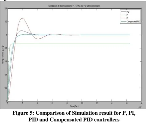
[image:5.595.315.557.110.302.2] [image:5.595.55.293.146.346.2]Using the above mentioned method, better values for Kp, Ki and Kd was found out and the simulation result is shown in Figure 5.
Figure 5: Comparison of Simulation result for P, PI, PID and Compensated PID controllers
The Kp, Ki, Kd values for different controllers, that were found out with the help of stability Boundary plots are given below.
For Proportional Control,
From the graph it is clear that, while using proportional control alone, a steady state error occurs. To avoid this we are adding an Integrator. Now, the parameters for Proportional Integral Control are,
Here the steady state error is minimized but system oscillates before settling. The proportional integral controller gives a sluggish output that means, it takes a lot of time to get settled. Also the overshoot is large. To avoid these problems, that is for faster settling we adds derivative controller with this controller as explained in chapter 1. Thus PID controller is introduced.
Also, for Compensated PID, the parameters are found to be,
From the bode plots shown in figure 6 it is clear that the phase margin is increased when using lead compensator [10, 11].
For stability analysis root locus method [10] is used, and the results are shown figure 7.
From the root locus plots, it is clear that the addition of lead compensator results a left shift in poles and thus the stability of the system is increased.
Figure 6: Comparison of bode plots of PID and Compensated PID controllers
Figure 7: Comparison of root locus of systems with PID and Compensated PID controllers
7.
CONCLUSION
The system identification is done by performing the Step Test. Tuning of parameters were done using the graphical method, Stability Boundary Locus Plot. The system with different controllers is then simulated to obtain the step response. The responses of P, PI, PID and PID controller with Lead Compensator are then plotted. The performance of compensated system is checked with the help of Bode Plot. It is found that at high frequency the system stability is marginally increased with the addition of Lead Compensator. The stability is then checked with the help of Root Locus plot. That results a shift in poles towards the left hand side of S-Plane, which means by adding the lead compensator the system shifts to the more stable region. Stability Boundary Locus method used here is found to be very easy to analyze compared to the conventional methods.
comparatively reduce the analyzing time. The lead compensator can be designed for non linear systems too. The highly non linear unstable systems like systems with magnetic levitation, spherical tanks etc can be linearized and can be stabilized with the use of lead or lag compensators.
8.
ACKNOWLEDGMENTS
At the outset, I express my gratitude to the ALMIGHTY GOD who has been with me during each and every step that I have taken towards the completion of this project. Also I wish to express my sincere thanks to my Department Faculties and the College Management who gave me support and provided me necessary facilities. I would like to convey my gratitude towards my parents and friends whose prayers and blessings where always there with me throughout this work
9.
REFERENCES
[1] G. Sridhar and K. Hrishikes, “Design and Implementation of Fractional Order PID Controller for Integer and Fractional Order Thermal Process”, International Conference on Computing and Control Engineering (ICCCE 2012), 12 & 13 April, 2012.
[2] Liptak K, “Process Control and Optimization”, Instrument Engineers' Handbook, Fourth Edition, Volume Two, pp 1169-1227, 103-110
[3] George Stephanopoulos, “Chemical Process Control”, An Introduction To Theory And Practice, Ptr Prentice Hall, New Jersey 07632,pp 70-75
[4] R. Zanasi, S. Cuoghi, “Analytical and Graphical Design of PID Compensators on the Nyquist plane”, IFAC Conference on Advances in PID Control PID'12, Brescia (Italy), March 28-30, 2012.
[5] Nusret Tan, Ibrahim Kaya, and Derek P. Atherton, “Computation of Stabilizing PI and PID Controllers”, Proc. of the 2003 IEEE Intern. Conf. on the Control Applications (CCA2003), Istanbul, Turkey.
[6] Radek Matušů, “Calculation of all stabilizing PI and PID Controllers”, International Journal of Mathematics and Computers in Simulation, Issue 3, Volume 5, 2011, pp 224-231.
[7] Nusret Tan, Ibrahim Kaya, and Derek P. Atherton, “A Graphical method for Computation of all Stabilizing PI Controllers”, Proc. of the 2003 IEEE Intern. Conf. on the Control Applications (CCA2003), Istanbul, Turkey.
[8] Weidong Zhang, Yugeng Xi, Genke Yang, Xiaoming Xu, “Design PID controllers for desired time-domain or frequency-domain response”, The Instrumentation, Systems, and Automation Society Transactions 41 – 2002, 511–520.
[9] Prof. Guy Beale, “Phase Lead Compensator Design Using Bode Plots”, International Conference on Mechatronics & Automation, George Mason University, Virginia.
[10]Amit Patel,and Gabriel A. RincónMora,"Stability Analysis: Bode Plots versus Root Locus", IEEE Georgia Tech Analog, Power, and Energy IC Research
[11]Nakhmani, Arie, "Generalized Nyquist Criterion and Generalized Bode Diagram for Analysis and Synthesis of Uncertain Control Systems", Electrical and Electronics Engineers in Israel, 2006 IEEE 24th Convention
[12]Yanqiu Cui,Yaning Yang, Tao Zhang, "Computer-aided design of lead compensator of control system via MATLAB", Electronic and Mechanical Engineering and Information Technology (EMEIT), 2011 International Conference on 12-14 Aug. 2011
[13]McCarthy, E.P., "Phase lead compensator design", Electronics Letters 11 Oct. 1990