Quantum Inspired Bee Colony Algorithm

(1)

http://dx.doi.org/10.4236/ojop.2015.43007

Quantum-Inspired Bee Colony Algorithm

Guorui Li1_,_{Mu Sun}2_{, Panchi Li}1

1_{School of Computer and Information Tsechnology, Northeast Petroleum University, Daqing, China}

2_{Beijing Branch of Daqing Oilfield Information Technology Company, Beijing, China}

Email: [email protected]

Received 15 March 2015; accepted 22 August 2015; published 25 August 2015

This work is licensed under the Creative Commons Attribution International License (CC BY).

http://creativecommons.org/licenses/by/4.0/

Abstract

To enhance the performance of the artificial bee colony optimization by integrating the quantum computing model into bee colony optimization, we present a quantum-inspired bee colony opti-mization algorithm. In our method, the bees are encoded with the qubits described on the Bloch sphere. The classical bee colony algorithm is used to compute the rotation axes and rotation an-gles. The Pauli matrices are used to construct the rotation matrices. The evolutionary search is achieved by rotating the qubit about the rotation axis to the target qubit on the Bloch sphere. By measuring with the Pauli matrices, the Bloch coordinates of qubit can be obtained, and the opti-mization solutions can be presented through the solution space transformation. The proposed method can simultaneously adjust two parameters of a qubit and automatically achieve the best match between two adjustment quantities, which may accelerate the optimization process. The experimental results show that the proposed method is obviously superior to the classical one for some benchmark functions.

Keywords

Quantum Computing, Bee Colony Optimizing, Bloch Sphere Rotating, Algorithm Designing

1. Introduction

(2)

other fields. However, the progress has been slow in the algorithm improvement. For the design of the control parameters, Ding Haijun et al. present an improved artificial bee colony algorithm for the solution to TSP prob-lem [9]. Kang Fei et al. propose a cultural annealing artificial bee colony algorithm [10]. Duan Haibin et al. present a new algorithm with application of the combination of artificial bee colony algorithm and quantum evolutionary algorithm [11].

As a new computing model, quantum computing catches wide attention of international and domestic aca-demics for its polymorphism, superposition and concurrency. At present, the fusion with genetic algorithm, im-mune optimization, paticle swarm optimization and other intelligent optimization model is successfully applied. In the real quantum system, the qubits are described on the Bloch sphere with two adjustable parameters. How-ever, in the existing quantum intelligent optimization algorithms, individuals are encoded by qubits described by unit circle with a single adjustable parameter. Evolutionary mechanism adopts quantum rotation gates and quantum non-gates, and it essentially rotates qubits about circle center, which only changes one parameter of qubits as well. Therefore quantum properties have not been fully reflected. Although Ref. [12] presents a quan-tum genetic algorithm based on the Bloch coordinates of qubit, however, this algorithm does not consider the match between two adjustment quantities, which means it doesn’t go along the shortest path when the current qubit moves towards the target qubit. As a result, the optimization performance is influenced.

This paper proposes a new individual coding evolutionary mechanism, which is different from the coding of quantum genetic algorithm in Ref. [12]. In this paper, we directly use qubits described on the Bloch sphere to code (not the qubits coordinates). The evolutionary search is achieved by rotating the qubit about the rotation axis on the Bloch sphere. This method can automatically achieve the best match between two adjustment quanti-ties of bee colony individual qubits. For the design of quantum-inspired bee colony algorithm, we elaborate de-sign principle and implementation programs of the algorithm. Taking benchmark functions extremum opti-mization as example, it shows that the proposed method obviously outperforms the classical one by comparison.

2. Bee Colony Algorithm

Assuming the number of bees is Ns, and the number of employed bees and onlooker bees are Ne and Nu, respectively. Individual dimension is D, and individual searching space is S=RD. The employed bee colony is

(

₁, ₂, ,

)

e

N

=

X X X  X and its initial the n-th generation colony is X

( )

0 and X

( )

n , respectively. The objective function is f S: →R+. Taking minimum optimization as example, the artificial bee colony algorithm can be described as follows:

(a) Randomly generating Ns solutions, where the i-th solution Xi is written as:

( )

(

)

min 0,1 max min

j j j j

i

X = X +rand X −X , (1)

where j=1, 2,,D. Calculate the target values, and then initialize X

( )

0 by the first Ne solutions;

(b) For the employed bee Xi in the current generation, the new position in its neighborhood can be obtained from the following equation:

(

)

j j j j j

i i i i k

V =X +φ X −X , (2)

where j∈

{

1, 2,,D

}

, k∈

{

1, 2,,N_e

}

, and k≠i, and ϕij is a random number in the range (0, 1);

(c) We use greedy selection operator to select the better ones in Vi and Xi for the next generation. This operator is denoted as T_s:S2→S, and its probability distribution is written as:

(

)

{

}

1,

( )

_{( )}

( )

_{( )}

,

0,

i i

s i i i

i i

f f

P T

f f

 <



= _{= }

≥ 

V X

X V V

V X ; (3)

(d) Using the strategy of roulette, randomly select an employed bee, and search a new position in its neigh-borhood. This operator is written as 1: e

N s

T S →S, and its probability distribution is written as:

( )

{

1

}

( )

1

( )

e

N

s i i m m

P T X =X = f X

∑

₌ f X ; (4)

(3)

(f) If algorithm meet the stopping criteria, it outputs fbest and the corresponding individual

(

x x1, 2,,xD

)

,

else go back to (b).

3. Quantum-Inspired Bee Colony Algorithm

This paper studies a new method of quantum-inspired searching with the fusion of bee algorithm. This method is named quantum-inspired bee colony algorithm (QIBC).

3.1. Description of Qubits on the Bloch Sphere

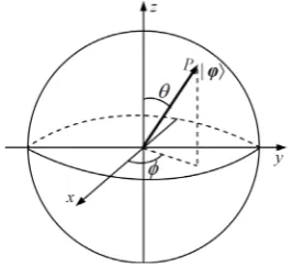
During the quantum computing, a qubit is a two-level quantum system which could be described in two-dimension complex Hilbert space. Based on principle of superposition, a qubit can be defined as:

i

cos 0 e sin 1

2 2

ϕ

θ θ

= +

ϕ , (5)

where 0≤ ≤θ π and 0≤ ≤φ 2π.

Owing to the continuity of θ and ϕ, a qubit can be in infinitely many different states and described by a point on the Bloch sphere. As shown inFigure 1.

3.2. The Rotation of Qubits about the Axis

In this paper, we create a search mechanism on the Bloch sphere which is used to rotate the qubit about the rota-tion axis to the target qubit on the Bloch sphere. The rotarota-tion can simultaneously change two parameters of a qubit, and automatically achieve the best match between two adjustment quantities, thus we can enhance the performance of optimization. The key to the above rotation is the design of rotation axis. The design method given by this paper can be expressed as the follows [13] [14].

Assuming P= p px, y,pz and Q= q q qx, y, z denote two points on the Bloch sphere respectively, the rotation axis Raxis about which P rotates to Q along the shortest path is the vector product of P and Q, namely,

axis= ×

[image:3.595.247.381.429.550.2]

R P Q. As shown inFigure 2.

Figure 1. A qubit description on the Bloch sphere.

[image:3.595.242.382.575.701.2]

(4)

Based on the principle of quantum computing, the rotation matrix makes the qubit rotate about arotation axis along the unit vector n= n n nx, y, z with radian of rotation δ, and it’s defined by

( )

cos i sin

(

)

2 2

δ δ

δ = − ×

n

R I n σ , (6)

where I is the unit matrix, and σ = σ σ σx, y, z, σ σ σx, y, z are Pauli matrices [15].

Therefore, on the Bloch sphere, the rotation matrix that rotates the ϕij

( )

t about Raxis

( )

i j, to ϕbj

( )

t can be described as follows:

( )

₍

_{( )}

₎

cos i sin ,

2 2

ij ij

ij axis

t t

i j

δ δ

= − ×

M I R σ . (7)

The rotation operation is given by

( )

ij t =Mij ij t

ϕ ϕ , (8)

where t is iteration step.

3.3. QIBC Coding Method

In QIBC, the individual coding adopts qubit based on the Bloch sphere. Let Ns denote population size, D denote the number of variables, and P= p1

( ) ( )

t ,p2 t ,,pNs

( )

t  denote the t-th generation colony. During in

itialization, the i-th individual can be coded as follows:

( )

1 2

(0) 0 , 0 , , 0

i =  i i iD 

p ϕ ϕ  ϕ , (9)

where i=1, 2,,Ns.

3.4. The Projection Measurement of Qubits

On the basis of the principle of quantum computing, by applying Pauli matrices to ϕ , we can get the Bloch coordinates of ϕ . The qubits projection measurement is denoted by the following equations:

0 1

1 0

x

x= = _ _

 

ϕ σ ϕ ϕ ϕ , (10)

0 i

i 0

y

y= = _ − _

 

ϕ σ ϕ ϕ ϕ , (11)

1 0

0 1

z

z= = _ _

−

 

ϕ σ ϕ ϕ ϕ , (12)

where i=1, 2,,Ns and j=1, 2,,D.

In QIBC, each qubit are regarded as three paratactic genes, each one contains three paratactic gene chains, and each of gene chains represents an optimization solution. Therefore, each entity represents three optimization solutions at the same time.

3.5. The Solution Space Transformation

)

Max 1 Min 1 2

ij j ij j ij

Z =_ −z + +z _ , (15)

where i=1, 2,,Ns and j=1, 2,,D. 3.6. Employed Bee Search

Taking minimum optimization as example, according to the value of target function, we rank the optimized population in descending order, and select the first Ne entities to compose employed bee colony. The rest of them compose onlooker colony. For the i-th employed bee p_i

( )

t , first of all, randomly select employed bees

( )

j t

( )

t between ϕid

( )

(

( )

)

(

( )

)

( )

(

( )

)

(

( )

)

ˆ , ˆ

ˆ ,

i i i

i

i i i

t f t f t

t

t f t f t

 <

 = 

≥ 

p p p

p

p p p , (16)

where,

( )

(

i

)

max

(

i

It is similar with employed bee search. First, we calculate selective probability of each employed bee with the equation as follows:

(

)

( )

1

( )

e N

i i m m

P p= p = f p

∑

₌ f p . (19)

To each onlooker bee, first, we select employed bee pi according to the roulette method, and in its neigh-borhood we search for new position ˆpi in the same method as the employed bee search. If ˆpi is better than

i

p , set p_i = pˆ_i , and set the number of searches Bas=0. If Bas is less than threshold Limit, set 1

Bas=Bas+ , otherwise, we initialize p_i and set Bas=0.

3.8. Algorithm Termination Criterion

To this algorithm, the termination criterion is the number of iterations. Whether it meets the pre-set accuracy or not, the algorithm will stop when the limited number of iterations reaches.

4. Analysis of Experimental Results

Taking functions extremum optimization as example, by comparing with bee colony [1], Bloch quantum genetic algorithm [12], elite genetic algorithm, quantum delta potential-based particle swarm optimization [16], we ve-rify the superiority of QIBC. All of algorithms use Matlab R2009a to implement on the computer (P-II 2.0 GHz) with 1.0 G memory.

4.1. Benchmark Functions

To verify the superiority of QIBC, the following ten Benchmark functions are used in this experiment. All of ten functions are for the minimum optimization, and X∗ is the minimum extreme value point.

(1) f₁

( )

X =

∑ ∑

D_i₌₁

(

i_j₌₁x_j

)

2 , −100≤xi ≤100, xi 0

∗₌

(6)

(2)

( )

(

)

(

)

1 ₂ 2 2 2 1 1 100 1 D

i i i

i

f x x x

−

+ =

=

∑

− + −

X , −100≤xi≤100, xi 1

∗₌

, f

( )

X∗ =0;

(3) 3

( )

4

(

( )

)

1

* 1 0,1

D

i i

f i x rand

=

∑

+

X , −100≤xi≤100, xi 0

∗₌

, f

( )

X∗ =0;

(4)

( )

2

1 1

0.2 cos 2π

4 20e e 20 e

D D

i

i x i xi

D D

f X = − − ∑= − ∑= + + , −100≤xi≤100, xi 0

∗ ₌

, f

( )

X∗ =0;

(5) 5

( )

(

)(

)

(

)

2 1

1 2

4 1

1 6

D D

i i i

i i

D D D

f x x x−

= =

+ −

= +

∑

− −

∑

X , 2 2

i

D x D

− ≤ ≤ , *

(

₁

)

i

x =i D− +i , f

( )

X∗ =0;

(6)

( )

2 6 1 1 cos 1 4000 D D jk jk k j y f y = =   = _ − + _  

∑∑

X , yjk =100

(

xk−x2j

) (

2+ −1 xj

)

2, −100≤xi≤100, xi 1

,

( )

(

)

(

)

0.25 0.1

2 2 2 2 2

, sin 50 1

g x y = x +y _ x +y + _

 ,

100 xi 100

− ≤ ≤ , xi 0

∗₌

, f

( )

X∗ =0;

(8)

( )

2 4

2 8

1 1 1

0.5 0.5

D D D

i i i

f x ix ix

= = =

   

= +_ _ +_ _

   

∑

X , −100≤xi ≤100, xi 0

∗₌

, f

( )

X∗ =0;

(9)

( )

2

9 1 1

1 cos 1 4000 D D _i i i i x

f X x

i

= =

 

= − _ _+

 

∑

∏

, −500≤xi≤500, xi =0,

( )

*

0 f X = ;

(10)

( )

(

2

(

)

10 10 1 10 cos 2π

D

i i

i

f X = D+

∑

₌ y − y ,

( )

, 1 2

2 2 , 1 2

i i

i

i i

x x y

round x x

 <

 = 

≥

 , −100≤xi≤100, xi=0,

( )

* 0 f X = .

4.2. Parameters Setting

For convenient comparison, based on the complexity of benchmark functions, we set up precision thresholds ε for each function. Only when optimization effect is less than the thresholds, the algorithm is call converges. In this experiment, the precision thresholds are set as follows. for f1, f6, ε =1.0; for f2 ε =10; for f3,

5 10

ε ₌ −

; for f4, f9, f10,

10 10 ε ₌ −

; for f5, 2 10

ε = ; for f7,

8 10 ε ₌ −

; for f8, 4 10

ε = . If the algorithm converges, the current optimization steps are called the number of iteration. If not, the number of iteration is equal to the pre-set limited number of iterations.

The dimensions of ten functions are set to D=30, and population sizes of five algorithms are equal to 40. For QIBC and BC, we have Ne =20, Nu=20, Limit=50. For BQGA, on the basis of Ref. [12], the initial value of rotation angle is 0.05π , and the mutation probability is 10-3

. For QDPSO, based on Ref. [16], the con-trol parameter is λ =1.2. For EGA, the crossover probability is 0.8, the mutation probability is 0.01. The li-mited number of iterations of five algorithms is G=104.

4.3. Comparison and Analysis of Simulation

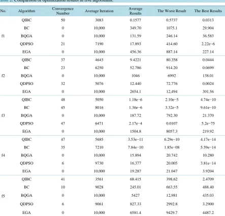
To enhance the objectivity of comparisons, each algorithm independently runs 50 times, and we have compari-sons of statistical results. The average time for each of iteration are shown in Table 1. To make comparisons be sufficient, besides showing the average results, the best and the worst ones are also are given. Comparison of the number of iterations, average iterations, and optimization results are shown inTable 2.

(7)

[image:7.595.89.541.105.276.2]

Table 1. Comparison of average time for each iteration (unit: second).

No. QIBC BC BQGA QDPSO EGA

f1 0.0281 0.0038 0.0216 0.0016 0.0026

f2 0.0219 0.0016 0.0095 0.0005 0.0015

f3 0.0223 0.0018 0.0100 0.0006 0.0015

f4 0.0218 0.0016 0.0103 0.0005 0.0014

f5 0.0221 0.0017 0.0098 0.0006 0.0014

f6 0.0596 0.0102 0.0429 0.0040 0.0126

f7 0.0245 0.0023 0.0270 0.0010 0.0011

f8 0.0222 0.0018 0.0104 0.0006 0.0015

f9 0.0176 0.0046 0.0116 0.0005 0.0003

f10 0.0183 0.0050 0.0178 0.0007 0.0005

Table 2. Comparison of optimization results in five algorithms.

No. Algorithm Convergence

Number Average Iteration

Average

Results The Worst Result The Best Results

f1

QIBC 50 3083 0.1577 0.5737 0.0313

BC 0 10,000 349.70 1075.1 29.904

BQGA 0 10,000 131.59 246.14 36.583

QDPSO 21 7190 17.893 414.60 2.22e−6

EGA 0 10,000 456.36 887.14 227.14

f2

QIBC 37 4643 9.4221 80.358 0.0444

BC 23 6250 52.786 914.20 0.0699

BQGA 0 10,000 1046 6992 138.01

QDPSO 32 5076 12.440 72.776 0.0024

EGA 0 10,000 2654.1 12,494 301.56

f3

QIBC 48 5050 1.18e−6 2.10e−5 4.74e−10

BC 45 8016 1.36e−6 3.32e−5 9.61e−10

BQGA 0 10,000 187.72 792.30 21.370

QDPSO 47 6471 2.17e−4 0.0107 5.2e−75

EGA 0 10,000 1504.8 8057.3 219.92

f4

QIBC 47 5685 3.53e−11 6.29e−10 4.17e−14

BC 35 7210 7.84e−10 1.85e−08 5.59e−14

BQGA 0 10,000 15.894 20.742 10.280

QDPSO 6 9730 16.377 20.005 3.81e−14

EGA 0 10,000 19.287 21.047 3.9204

f5

QIBC 41 3561 68.415 398.62 2.4709

BC 10 9028 245.01 663.55 488.40

BQGA 0 10,000 5427 12,981 435.03

QDPSO 6 9061 827.33 2992.8 3.2900

[image:7.595.92.536.293.718.2]

(8)

Continued

f6

QIBC 49 2467 0.1926 8.9054 1.25e−09

BC 28 5838 17.966 106.97 3.47e−08

BQGA 0 10,000 491.21 829.02 196.59

QDPSO 0 10,000 171.47 351.05 8.8842

EGA 0 10,000 22,127 355,958 978.91

f7

QIBC 49 5763 3.39e−09 1.69e−07 0

BC 36 8354 3.67e−08 1.45e−6 1.49e−10

BQGA 0 10,000 110.73 169.67 32.058

QDPSO 32 8640 0.4312 9.2145 2.42e−19

EGA 0 10,000 164.55 231.46 93.272

f8

QIBC 50 5454 1412 5700 61.335

BC 0 10,000 50,112 69,884 33,193

BQGA 0 10,000 4910.5 12,882 1006.1

QDPSO 50 7392 2003 5300 200.81

EGA 0 10,000 7843.8 38,137 4291.6

f9

QIBC 50 2162 8.65e−17 3.33e−15 0

BC 36 3424 0.0033 0.0221 0

BQGA 12 7780 0.0239 0.1275 0

QDPSO 29 5040 0.0062 0.5136 0

EGA 0 10,000 3.1224 7.3366 1.6101

f10

QIBC 50 2606 1.13e−14 1.13e−13 0

BC 49 6290 4.03e−12 1.89e−10 0

BQGA 0 10,000 172.42 416.64 26.023

QDPSO 6 9284 7.3553 15.882 0

EGA 0 10,000 822.60 1298.1 455.30

larger.

In Table 2, for the ability of optimization, obviously, QIBC is better than QIBC, BQGA is better than EGA. QDPSO is worse than QIBC, but it’s better than BQGA, and it’s similar to BC. For the optimization perfor-mance of five algorithms, we rank them in descending order as QIBC, BC, QDPSO, BQGA, EGA.

For the above results, we present the following analysis. Firstly, we introduce the coding mechanism of qubit with three chains, and it effectively enhances the ergodicity of algorithm to solution space. Based on the geome-tric properties of the Bloch sphere, this mechanism can enlarge the number of global optimal solutions and the probability of attaining global optimal solutions. That is the reason why these two algorithms are better than their classical ones respectively. Secondly, QIBC has a better performance of optimization than BQGA, because they adjust qubit in the different ways.

In BQGA, qubits are updated by directly adjusting θ and ϕ with the same adjustment amount (namely

θ ϕ

(9)

[image:9.595.91.538.105.197.2]

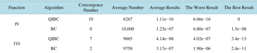
Table 3. Comparison of optimization results in QIBC and BC.

Function Algorithm Convergence

Number Average Number Average Results The Worst Result The Best Result

f9

QIBC 10 6267 1.11e−16 6.66e−16 0

BC 0 10,000 1.23e−07 6.80e−07 1.5e−08

f10

QIBC 7 9065 4.14e−08 4.02e−07 3.4e−13

BC 2 9758 3.17e−07 1.90e−06 2.4e−11

the shortest. Although it does’t adjust two parameters of qubit directly, it achieves the best match between ∆θ and ∆ϕ automatically and accurately. Hence, this method has better optimizing efficiency than classical ones.

It’s also worth pointing out that, although the QIBC has better optimizing performance, the complexity of this algorithm is obviously higher than classical ones. Comparing with classical ones, the QIBC needs some extra operations, such as calculating rotation axis, rotation angel, rotation matrices and the solution to space transfor-mation. Considering run time and optimizing performance, QIBC earns better optimizing efficiency by sacrific-ing runnsacrific-ing time, which is the same as No Free Lunch. For many off-line optimizsacrific-ing tasks which may ignore running time, the QIBC has wide application prospects.

We need investigate and study the influence after dimensions and parameters change. Taking f9 and f10 as example, while D=100, population size is Ne =Nu =40, and Limit=100,

4 10

G= . Precision threshold of f9 and f10 is

10

10− . The QIBC and the BC run 10 times respectively. Optimization results is shown in

Table 3.

As the results are shown, for the high-dimensional optimization problems, the proposed algorithm also shows its better performance than classical ones.

5. Conclusion

We present a quantum-inspired bee colony optimization algorithm. In proposed method, the bees are encoded with the qubits described on the Bloch sphere. The population evolutionary is achieved by rotating the qubit about the rotation axis on the Bloch sphere. The experimental results show that, the method of qubits coding on the Bloch sphere and the method of bee updating which can achieve the best match between two adjustment quantities of qubit parameters by rotating about the rotation axis, can truly enhances the performance of the in-telligent optimization algorithm.

Acknowledgements

This work was supported by the Natural Science Foundation of Heilongjiang Province, China (Grant No. F2015021), the Youth Foundation of Northeast Petroleum University (Grant No. 2013NQ119) and the Science Technology Research Project of Heilongjiang Educational Committee of China (Grant No. 12541059).

References

[1] Karaboga, D. (2005) An Idea Based on Honey Bee Swarm for Numerical Optimization. Technical Report-TR06, En-gineering Faculty, Computer EnEn-gineering Department, Erciyes University, Kayseri.

[2] Bahriye, A. and Dervis, K. (2012) A Modified Artificial Bee Colony Algorithm for Real-Parameter Optimization. In-formation Sciences, 192, 120-142. http://dx.doi.org/10.1016/j.ins.2010.07.015

[3] Xiang, W.L. and An, M.Q. (2013) An Efficient and Robust Artificial Bee Colony Algorithm for Numerical Optimiza-tion. Computers & Operations Research, 40, 1256-1265. http://dx.doi.org/10.1016/j.cor.2012.12.006

[4] Li, G.Q., Niu, P.F. and Xiao, X.J. (2012) Development and Investigation of Efficient Artificial Bee Colony Algorithm for Numerical Function Optimization. Applied Soft Computing, 12, 320-332.

http://dx.doi.org/10.1016/j.asoc.2011.08.040

[5] Karaboga, D., Akay, B. and Ozturk, C. (2007) Artificial Bee Colony (ABC) Optimization Algorithm for Training Feed-Forward Neural Networks. Modeling Decisions for Artificial Intelligence, 4617, 318-329.

(10)

[6] Karaboga, N. (2009) A New Design Method Based on Artificial Bee Colony Algorithm for Digital IIR Filter. Journal of the Franklin Institute, 346, 328-348. http://dx.doi.org/10.1016/j.jfranklin.2008.11.003

[7] Rao, R., Narasimham, S. and Ramalingaraju, M. (2008) Optimization of Distribution Network Configuration for Loss Reduction Using Artificial Bee Colony Algorithm. International Journal of Electrical Power and Energy Systems En-gineering, 1, 709-715.

[8] Singh, A. (2009) An Artificial Bee Colony Algorithm for the Leaf-Constrained Minimum Spanning Tree Problem. Ap-plied Soft Computing, 92, 625-631. http://dx.doi.org/10.1016/j.asoc.2008.09.001

[9] Ding, H.J. and Li, F.L. (2008) Bee Colony Algorithm for TSP Problem and Parameter Improvement. China Science and Technology Information, 25, 241-243.

[10] Kang, F., Li, J.J. and Zu, Q. (2009) Improved Artificial Bee Colony Algorithm and Its Application in Back Analysis. Water Resources and Power, 27, 126-129.

[11] Duan, H.B., Xu, C.F. and Xing, Z.H. (2010) A Hybrid Artificial Bee Colony Optimization and Quantum Evolutionary Algorithm for Continuous Optimization Problems. International Journal of Neural Systems, 20, 39-50.

http://dx.doi.org/10.1142/S012906571000222X

[12] Li, P.C. (2008) Quantum Genetic Algorithm Based on Bloch Coordinates of Qubits and Its Application. Control Theo- ry & Applications, 25, 985-989.

[13] Li, P.C. and Lin, J.J. (2012) Chaos Quantum Immune Algorithm Based on Bloch Sphere. Systems Engineering and Electronics, 34, 2592-2598.

[14] Li, P.C., Wang, Q.C. and Shi, G.Y. (2013) Quantum Particle Swarm Optimization Algorithm Based on Bloch Spheri-cal Search. Chinese Journal of Computational Physics, 30, 454-462.

[15] Giuliano, B., Giulio, C. and Giuliano, S. (2004) Principles of Quantum Computation and Information (Vol. I: Basic Concepts). World Scientific, Singapore, 100-112.