The A-r-Star (
) Pathfinder
Daniel Opoku
Department of Electrical andComputer Engineering North Carolina Agricultural and
Technical State University
Greensboro, NC 27411
Abdollah Homaifar
Department of Electrical andComputer Engineering North Carolina Agricultural and
Technical State University
Greensboro, NC 27411
Edward Tunstel
Research and Exploratory Development Department Johns Hopkins University AppliedPhysics Laboratory
Laurel, MD 20723
ABSTRACT
This paper presents a variant of the A-Star ( ) pathfinder for robot path planning called (pronounced A-r-Star)and demonstrates that the algorithm outperforms in a uniformly gridded sparse world and gives performance matching that of in a uniformly gridded cluttered world. This algorithm is simple to implement and understand. It alsohighlights the performance advantages of the algorithm and proves its properties experimentally and analytically (where appropriate). Some challenges affecting the performance of have been presented and some solutions to these challenges have been developed and implemented. The performance of has been compared to running on both uniform and multi-resolution grids of different world scenarios. Results show that on a sparse high-resolution uniform grid world ’s search speed scales well and it outperforms by an exponential factor.
General Terms
Artificial Intelligence, Algorithms, Pathfinder, Graph Search
Keywords
Pathfinder, Path Planning, A-r-Star, A-infinity-Star, Multi-resolution, Path Smoothing
1
INTRODUCTION
Many researchers have studied path planning for robotics [1] using occupancy grid map representations of the world. In this context, the world is usually considered as a finite area within which a robot will operate. Here the map is represented as a mesh of nodes spread over the continuous space of locations in the world. Each node, of the mesh is parameterized by its occupancy , or probability of being occupied by an object or obstacle. Thus, for the 2D binary occupancy grid such as that used in this paper, expresses an occupied node and expresses an unoccupied node. For robotic path planning, the 2D grid is often used to represent a slice of a 3D world. The path planning problem is stated as: Given a start node and goal node belonging to a given grid world, find the shortest unblocked path connecting them. This paper presents a novel algorithm, (pronounced A-r-Star), a modified version of the pathfinder for path planning in a uniform grid world. This new algorithm outperforms path planning in a sparse uniformly gridded world and matches in a cluttered world. The algorithm essentially interweaves the building of a non-uniform grid out of a uniform gridded world with path-finding. When given a uniform grid world, decimates the nodes within a given radius/range (r) and forms bigger nodes out of them. It has been shown both experimentally and analytically (where appropriate) that
possesses most of the desirable features of . Besides, some challenges that affect the performance of have been identifiedand some strategies to mitigate them have been developed thereby bringing ’s performance close to optimal. The performance of has been compared to running on both uniform grids and multi-resolution grids of different world scenarios. Results show that, when running on sparse high dimensional, high resolutiongrid worlds, ’s performance scales well (linearly) with increasing grid size and outperforms by an exponential factor.
The rest of the paper is organized as follows. Section 2 presents a literature review of related pathfinders. Section 3presentsthe motivation for developing the algorithm followed by the description of in Section 4. The new pathfinder is presented in Section 5 followed by the description of its properties in Section 6, challenges in Section 7 and suggested solutions in Section 8. Section 9 presents results of simulation experiments highlighting algorithm properties followed by conclusion and future work in Section 10.
1.1 Nomenclature
= finite set of all nodes to be searched, ; set of all unoccupied/unblocked nodes;
set of all blocked nodes;
set of all the nodes that ever make it to the list, thus ;
set of all the nodes on the list, thus ;
cardinality of set ; an individual node, ;
cost of traversing from node to its neighbor ; = starting node;
= goal node
cost of moving from to ;
= estimated heuristic cost of moving from node to ;
= set of all the successors of ; = set of all the predecessors of ;
parent of ,
2
LITERATURE REVIEW
overestimates the actual minimal cost of reaching the goal (i.e., it is admissible) then is admissible and thus always optimal (i.e., it will explore/expand the minimum possible number of nodes necessary) [3]. Subsequently, the use of the algorithm for path planning in both robotics and video games has increasingly gained popularity. To use for path planning given a 2D map of the environment, one first reduces the robot size to a point robot and enlarges the obstacles in the environment by the radius of the robot’s cross-section (using configuration space computation) [4][5]. This ensures that the robot can traverse any path of empty nodes returned by the search algorithm without colliding with an obstacle. Given start and goal nodes, the algorithm searches through continuous obstacle free 4-connected or 8-connected nodes (depending on application) for a path with minimum cost from the start to goal, where the cost of a path is the sum of the costs of its arcs or segments.
The algorithm has limitations that make its application to some especially large grid worlds unattractive. One of the limitations is that the search time increases exponentially with increasing grid size. This is so because finding adjacent nodes with lowest cost, can be time consuming due to the growing size of the OPEN list, a data structure storing the nodes to be evaluated. Also, insertion of a node onto the OPEN list involves computation of the node’s associated costs which makes searching through many nodes very computationally expensive. Various solutions have been suggested in literature to mitigate this challenge such as the following [6]:
(i)The OPEN list can be implemented with a priority queue data structure sorted according to the cost function, ). Thus, determination of the node with lowest cost reduces to simply popping the priority node of the queue. The priority queue creation takes time[7]and thus the time scales linearly with fast growing OPEN lists;
(ii) Instead of using a list/queue, if memory is not a limiting resource, the OPEN list can be implemented with arrays using memory allocation and access routines to reduce the time it takes to find the node with lowest cost function to ;
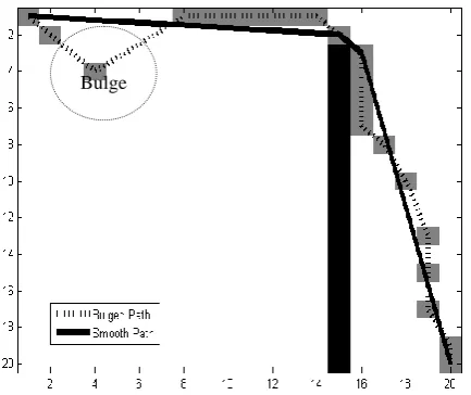
(iii) A low resolution/coarse grid can be used with fewer nodes to search, and hence permits faster run time. However, coarse discretization of the continuous world can result in the creation of unrealistic paths where an obstacle is close to the boundary (see Figure 1) and it can also place a node beyond reach especially in a cluttered environment (see Figure 2);
(iv) The use of a multi-resolution grid representation of the environment is another way to solve this problem in a sparse world. This involves preprocessing the world into a non-uniform grid representation such as quadtrees. Using this approach involves an initially high capital cost in building the world map. However, once that is completed, it yields good run time performance in terms of search speed. Hence, this approach is suitable for planning in a static world.
Regarding solution (iv) described above,small obstacles and protrusions from irregular obstacles in a region result in the creation of small obstacle nodes due to the recursive nature of the quadtree. These fragment the free space, giving rise to an undesirable increase in the depth of the quadtree and the number of leaf nodes and consequently increasing the cost of the search [8].
usually returns a ‘kinky’ path (path with many unnecessary turns) making its direct usage by a robot impractical. Post smoothing and interleaved smoothing techniques are usually employed to remove these kinks [9].
, being an offline search technique works on the assumption that the world is fully known and unchanging. Whenever the robot observes a discrepancy between the given map and the navigation world that affects the planned path (e.g., a node on the path is unexpectedly blocked), it has to re-plan a new path starting anew from its current position. This becomes unbearable in even a moderately slow changing environment with high-dimension grid. Despite its optimality, the gross inefficiency accumulating from multiple re-plans may require a high-performance computer for real-time operation.
In effect, is best suited for offline path planning in a static world. This has prompted the development of a vast number of incremental path planning techniques. Anthony Stentz’s [10] is by far the most popular among the incremental search techniques. is capable of planning paths across the spectrum of fully known to unknown environments in an efficient, optimal, and complete fashion. As in , the environment is modeled as a graph, where each node represents a robot state (e.g., a location in a house), and each arc represents the cost of moving between two states (e.g., distance to travel). initially exploits the available information contained in the map (if any) to plan a path from the goal to the robot’s position in a way similar to . The robot then starts navigating using this path while simultaneously observing its environment through its sensors. If the robot discovers that the path is blocked (path changes are handled as arc cost changes), it calls on to plan a new path. propagates information about the arc cost changes minimally to all affected nodes in the graph to compute a new optimal path[11]. The robot repeats this process until it reaches the given goal or accrues enough information to establish that the goal is unreachable. This makes its application in a dynamic world attractive. However, the initial planning of a takes longer time since it operates as a Breadth-First Search. [12] is an extension of that uses heuristics to focus the search to significantly reduce
(a) Continuous world (b) The course
gridded world
[image:2.595.313.549.83.189.2](c)The fine gridded world
Figure 1: How increasing resolution can help graph search algorithms.
(a) Continuous world
(b) The course gridded world
(c)The fine gridded world
[image:2.595.319.546.378.470.2]the total time required for both the initial path calculation and subsequent re-planning operations thereby making the algorithm a full generalization of for dynamic environments. applies to robot navigation in unknown terrain, including goal-directed navigation in unknown terrain and mapping of unknown terrain[13]. The algorithm is easy to understand and analyze;it implements the same behavior as Stentz’s but is algorithmically different. The [14,15] algorithm is a variant of that uses interpolation to improve the smoothness of the path returned both in the planning and the re-planning phase.
is a fast version of that achieves exponential speedup in a sparse grid map. Itachieves this by interleaving path finding with multi-resolution gridding. This reduces the number of nodes that need to be explored in a sparse grid map, the computational intensity and hence the speedup.
3
MOTIVATION
Map building using fixed node decomposition (i.e., the continuous world is tessellated into a discrete approximation of the continuous map) is inexact resulting in the loss of narrow passages in this transformation. The higher the resolution of the grid, the closer the approximation is to the continuous world. But increasing the resolution introduces more free nodes and increases the search space leading to a sparse grid. The map of most indoor environments can be considered sparse if decomposed into nodes of high resolution. Applying to a sparse grid is not attractive since its run time is on the order . To solve this problem, multi-resolution gridding [8, 16] is usually adopted so that areas around obstacles receive high resolution gridding and areas far from obstacles are represented by much courser gridding. But building multi-resolution/adaptive grids requires more work in the decomposition than building uniform/fixed node grids. Besides, determining which node a given position belongs to and finding the neighbors of a given node in a multi-resolution grid is a non-trivial task [17]. The motivation is therefore to develop a complete and correct search algorithm that can plan paths in dimension, high-resolution grid maps faster. This will enable us to handle large grid sizes and thus encourage increasing the resolution of the grid without the need for multi-resolution.
4
A-STAR (
) ALGORITHM
DESCRIPTION
is a best-first search algorithm that finds the least costly path from an initial configuration to a final configuration in a given finite and static grid world. It uses an estimate of the start distance and heuristic estimation of the goal distance to define a cost/sorting function, (i.e., ). Generally, the algorithm maintains two lists namely list and list. The list is a priority queue of all the states which have at least one of their predecessors already explored and as such are potential candidates for next exploration. The list holds the candidates that have been explored at least once (and often the blocked nodes). The algorithm starts with an empty list and populates it with the starting node. At the beginning of every iteration, the node with the minimum cost , is popped from the list. If that is the goal node, the algorithm terminates and follows back pointers to extract the shortest path (i.e., the path with minimum cost). Else, that node is placed on the list and then expanded (i.e., the neighbors are generated and conditionally placed on the OPEN list).It proceeds with the iteration until
the goal node is expanded or the list becomes empty in which case it returns ‘no path found’. The pseudocode is shown in Algorithm 1.
5
A-R-STAR (
) ALGORITHM
5.1 Definitions
Node Distance of
from is defined as the fewest number of nodes that will be touched by a straight line connecting s and (see Figure 3). This is equivalent to the distance from to using the ‘chessboard’ distance metric. Thus, two nodes with different Euclidian distances can have the same node distances.Level-R-Neighbors of a node
comprise all nodes within node distances equal to R from . This implies that the Level-1-Neighbors of are its 8 contiguous neighbors (see Figure 3). Here Rrefers to the radius of the ‘ball’ (a box in the case of square grid) formed by connecting the centers of all Level-R-Neighbors.{1}
{2}
{3} {4}
{5} {6}
{7} {8} {9}
{10} {11}
{12} {13} {14}
{15} {16}
{17} {18} {19} {20}
{21} {22}
{23} {24} {25}
{26} {27}
{28}
{29}
{30} {31} {32}
{33} {34} {35} {36} {37}
5.2 Algorithm Description and
Implementation
[image:4.595.327.533.163.329.2]The algorithm is a modified version of the algorithm that interweaves node decimation with path-finding in a uniform grid/mesh. For a given node, counts only immediate nodes (4- or 8- connected nodes) as its neighbors. This implies that even when all the nodes in a particular area are similar, it will still do some computation for all of them. The effect is that, if an obstacle blocks the direct line of sight close to the goal, the number of nodes needed to be explored more than doubles (see Figure 4) which translates into increasing the search time.
Figure 3: Showing the Level-R-Neighbors for a given node All the nodes at a given level bear their node distance and is the Euclidean distance and is the node distance ( ). Here .
Using the idea from non-uniform mesh building[18], a cluster of nodes with similar characteristics can be represented with a bigger node with minimal loss of information (see Figure 5).
Figure 4: Showing (a) how responds to an obstacle; (b) ‘kinky’ path returned by and smooth path after post process. The circles indicate the nodes that were explored before the path was found.
The algorithm therefore allows collapsing of such nodes into a single node with properties that are commensurate with the union of those nodes (see Figure 5). For multi-level terrain, one will use a distance transform [19, 20] to identify changes in the nodes; but for the binary occupancy grid such as the one used in this paper, the task reduces to identifying the nearest obstacle to the current node. The overall effect is reduction in the number of nodes needed to be explored,
computation cost and increased search speed in a sparse uniform gridded world. The ‘star’ in the name does not suggest that it always finds an optimal path, it is just intended to retain its resemblance toits namesake, . The r stands for radius (range) defined as the maximum allowable radius (in node distance) of a ‘ball’ of nodes that can be counted as the neighbors of a given node (see Figure 3). Thus, only Level-R-Neighbors are considered during the search where .
Figure 5: The nodes at Level-1 to Level-3 decimated to form one big node with the original Level-4-Neighbors of
now forming the neighbors of the new node. Let the node distance fromthe closestobstacle node to a given node be , then at the end of the search
. Implementation-wise, this is achieved by searching for the minimum R such that at least one of the Level-R-Neighbors of a node being expanded belongs to the set of blocked nodes. Then all nodes in the neighborhood of such that are tagged as skip nodes ( ) and nodes such that are returned as the Level-R-neighbors.The pseudocode for the algorithm is similar to that of with two modifications. The first modification is done to the Expand subroutine and the resulting algorithm is referred to as . This is achieved by replacing the lines {21} to {28} in Algorithm 1 by the lines in Algorithm 2.
{21} {22}
{23} {24}
{25} {26} {27}
{28}
{29}
{30} and {31} {32}
{33} {34} {35}
{36} {37} {38}
[image:4.595.65.278.202.376.2] [image:4.595.76.268.472.631.2]Note that nodes that are tagged skip will never make it to the list (Algorithm 2 line {30}) but a node might make it to the list before being tagged as skip. Thus, in the algorithm, tag open dominates/overwrites tag skip. The second modification is to switch the tag dominance to skipdominating open. Thus, nodes that made it to the list from one node before being tagged as skip from another node will not be expanded (i.e., they will stay on the list till the algorithm terminates). The resulting algorithm after the last modification is called the algorithm. The pseudocode can be derived from the by inserting the lines in Algorithm 3 after the line {10} in Algorithm 1.
{11} {12}
Algorithm 3: Second modification resulting in the
5.3 Finite Radius (r) vs. Infinite Radius (∞)
The choice of can be fixed from the start of the algorithm to a finite value. For example, choosing reduces the algorithm to which is essentially . But choosing an appropriate finite value for requires absolute knowledge of the environment since the choice of affects the performance of the algorithm. The simplest solution is to allow the algorithm toevolve and discover the valueof r during the search. This is achieved by pegging the value of r at infinity (i.e., choosing ). This leads to what is referred to as the (A-Infinity-Star). Here, infinity (∞) is defined as where is the radius of the biggest ‘ball’ of continuous free nodes available in the search space. It is trivial to derive that for an grid world, always holds (strictly less because the node under consideration cannot be counted as part of the radius and is undefined for ).5.4 Choice of Level-R-Neighbors Generator
(LRNG)
TheLRNG function is responsible for generating Level-R-Neighborsof a given node . A good choice of the LRNGfunction should return at everyLevel-R, all and only the nodes at radius R from as the Level-R-Neighbors of . This is a necessary condition for to be complete and correct. On square grids, choosing the LRNGis a trivial task but this is not trivial when other geometric shapes are used for the gridding.
5.4.1
Theorem 1
If the Level-R-Neighborhoodgeneration function of at every Level-Rreturns all and only the nodes at radius from s for then the algorithm is complete and correct.
Proof:Let us assume the contrary that the path, returned by the algorithm is incorrect, thus there exists at least one between and , , such that . This will imply that a blocked node got expanded by the algorithm which contradicts the line of Algorithm 2 and therefore cannot be true. Similarly, let us assume that a path actually exists but did not find a path. This will imply at a certain Level-R, the algorithm failed to return a node and hence assumed there was not a path available. This is the necessary condition for a function to qualify as an LRNG and hence poses a contradiction that cannot surface.
6
PROPERTIES OF THE A-R-STAR
(
) ALGORITHM
6.1 Completeness
Like , the algorithm is complete meaning it will find a path if one exists between the start and the goal node. The condition for completeness solely depends on the as stated in Theorem 1.
6.2 Correctness
The correctness property holds for the algorithm. This implies that if does return a path for a given starting and ending node, then that path is a truly unblocked path (that is, the path exists and is correct).
6.3 Termination in Finite Time
The use of the CLOSED list and the tagging ensure that expands (or tags) every node once. Since the world is an grid, where is finite, it is implicit that the algorithm will terminate in finite time.
6.4 Convergence to
A*
The performance of the (and for that matter ) approaches that of for worlds with increasing clutter. Let us define a perfectly cluttered 2D world as a grid configuration such that every Level-1-Neighbor of
contains at least one . Given a perfectly cluttered world, the will be forced not to tag any node as skip. Thus, will implicitly operate as which is essentially .
6.4.1
Theorem 2
In a perfectly cluttered world, and converge to for all positive integer values of .
Proof:Assume the set is a perfectly cluttered 2D environment. Then every Level-R-Neighborhood of a free cell will contain at least one and thus ; from subsection 5.2,
for all nodes. But the runs at Level-R = 1 throughout the search and so it is intuitive that after the search, and hence the proof.
6.5 Any Angle Path Planning
Most of the grid-based path planning algorithms that operate on a 2D world use discrete state transitions that are artificially constrained to a small set of possible headings angles (e.g., etc.). The ramification is that the path returned by even the optimal grid planner will not be the shortest possible continuous path (see Figure 4). The algorithm is not constrained to a finite set of angles. This means that it sometimes returns a more natural and smooth path than . The algorithm under sparse conditions can therefore be considered as an‘any angle path planner’.
6.6 Reaction to Obstacle
The algorithm reacts to an obstacle by planning in small steps till it avoids the obstacle. This mimics intuitive navigating behavior. Much caution is taken when navigating close to an obstacle than when navigating far from an obstacle.
6.7 Definitions
. A continuous path is an unbroken curve drawn from the center of to the center of without passing through a blocked node. Let be the set of all continuous paths linking the centers of and , and let be a specific continuous path linking the centers of and . Define
. Thus, for a given grid map, if (i.e., there is an unobstructed straight line path from to ) then
= a straight line.
7
CHALLENGES OF THE A-R-STAR
(
) ALGORITHM
7.1 Bulges
usually returns a path with in it (see Figure 6). This is a major challenge to the performance of . Given two nodes, and , if and
straight line, then is called a path and, in general, any
[image:6.595.60.277.406.588.2]is said to be a bulged path. This definition implies that a ‘kink’ is a type of bulge (see Figure 4). There are two main causes of bulges in ; namely, angular constraint (kinks)and premature tagging. Angular constraint occurs around obstacles where the algorithm navigates in small steps; the navigation angles are thus artificially constrained to a small set of angles. Premature taggingoccurs due to local minima. The greedy heuristic of is initially drawn into a local minimum. This is accompanied by the tagging of nodes as skip. When the algorithm bounces back from the local minimum, these nodes which were prematurely tagged as skip are not considered for expansion and this creates a bulge.
Figure 6: An example of a path planned by highlighting the challenges posed by bulges and bulge elimination using post smoothing.
7.2 Non-optimality
Due to bulges, the path returned by is not always optimal. Bulges introduce extra cost into the sorting function by increasing the estimated goal distance thereby placing some nodes at a disadvantage. The goal distance becomes dependent on the configuration of the obstacles in the environment. Consequently, does not always imply during the search (where is the actual optimal path between and ). Thus, unlike the algorithm, does not always guarantee an optimal path.
8
PROPOSED SOLUTIONS TO THE
CHALLENGES
8.1 Bulge Removal: Post Dissociative
Smoothing (PDS)
A Post Dissociation Smoothing (PDS) algorithm similar to that outlined in [9]has been developed and implemented to eliminate the bulges in the path returned by . This shortens the path and gets it closer to the shortest possible path. Algorithm 4 shows the pseudocode for the PDS. Both and are derived from the Bresenham line drawing algorithm similar to that in [9].
{1}
{2} {3}
{4} {5} {6} {7}
{8} {9}
{10} {11}
{12} {13}
{14} {15} {16}
Algorithm 4: Post Dissociative Smoothing Algorithm
8.2 Non-optimality: Interleave Smoothing
with Post Dissociative Smoothing
(IS-PDS)
Some path configurations cannot be smoothed into the shortest possible/optimal path. To increase the chances of returning a path that can be smoothed to optimal, the search has been interleaved with the smoothing algorithm. This is similar to the idea in [9]. The post dissociative smoothing is then applied to the path as a post process. Note that PDS can be applied iteratively from goal to start and vice versa until subsequent application does not shorten the path by a distance greater than (where is a user defined threshold). This results in Interleave Smoothing with Iterative Post Dissociative Smoothing (IS-IPDS). To implement the interleave smoothing; replace the function of the algorithm with Algorithm 5.
9
SIMULATIONEXPERIMENT
RESULTS
In this section,simulation experiments have been used to highlight the properties of the / pathfinder and show its performance as compared to on different world scenarios using both uniform and non-uniform gridding. The simulations were developed using MATLAB (2011b, The MathWorks) running on PC with the Windows 8 OS. The simulation world comprises a grid of size (which amounts to 65536 nodes). The performance parameters include: (a) Search Time: the time it takes to plan a path; (b) Number of cells on OPEN list: the total number of cells that ever made it to the OPEN list throughout the search; (c) Number of cells explored: the number of cells that were actually explored before the goal was reached. In addition, example pathfinder applications to maze solving and indoor navigation are presented.
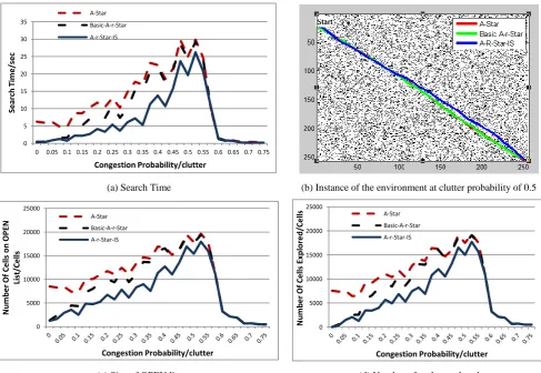
9.1 Effect of Congestion/Clutter on Performance of A-Star and Basic A-r-Star and A-r-Star
In the first experiment, the simulation environment was populated with obstacle nodes having congestion/clutter probability varied from 0 to 0.75, and with and . Results are shown in Figure 7. It was observed that no path existed beyond congestion probability of 0.6. Since over half of the nodes are occupied, it makes sense that searching from one extreme corner of the world to another will not have an unblocked path. Secondly, as the clutter increases, the number of free nodes decreases and this explains the sudden reduction in the graphs of performance parameter values after congestion probability of 0.55. The simulation results in Figure 7 demonstrate that and converge to beyond some degree of congestion (Theorem 2).(a) Search Time (b) Instance of the environment at clutter probability of 0.5
[image:7.595.52.540.398.734.2](c) Size of OPEN list (d) Number of nodes explored
Figure 7: The effect of congestion/clutter on , and operating on a uniform grid world 0
5 10 15 20 25 30 35
0 0.05 0.1 0.15 0.2 0.25 0.3 0.35 0.4 0.45 0.5 0.55 0.6 0.65 0.7 0.75
Se
arch
Ti
m
e
/s
e
c
Congestion Probability/clutter A-Star
Basic-A-r-Star
A-r-Star-IS
0 5000 10000 15000 20000 25000
Num
be
r
O
f
C
e
lls
on
O
P
EN
Li
st
/C
e
lls
Congestion Probability/clutter A-Star
Basic-A-r-Star
A-r-Star-IS
0 5000 10000 15000 20000 25000
Num
be
r
O
f
C
e
lls
E
xpl
ore
d/
C
e
lls
Congestion Probability/clutter A-Star
Basic-A-r-Star
A-r-Star-IS
{38} {39}
{40}
{41} {42}
{43} {44} {45} {46}
{47}
{48}
{49} {50}
{51} {52} {53} {54}
9.2 Effect of Changing Obstacle Configuration on Performance of A-Star and Basic A-r-Star
and A-r-Star (Sliding Obstacle)
This simulation experiment shows thatchanging the obstacle configuration has little effect on performance whereas it can drastically degrade the performance of operating in a sparse world such as the one shown in Figure 8 (b). The obstacle is assumed to be a long rigid wall in the environment separating the and . The horizontal position of this obstacle was varied from 11 to 231 and the performances of the pathfinders were recorded after each run.
(a) Search Time (b) Instance of the environment
[image:8.595.54.546.148.477.2](c) Size of OPEN list (d) Number of nodes explored
Figure 8: The effect of changing obstacle configuration on , and operating on a uniform grid world
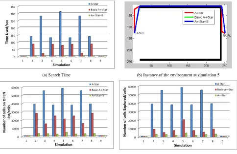
9.3 Effect of Changing
and
Configuration on Performance of A-Star and Basic
A-r-Star and A-r-A-r-Star in the presence of a Concave Obstacle
This simulation experiment shows that can better handle a large concave obstacle than . The obstacle is assumed to be a large rigid concave wall in the environment separating the and . Table 1 shows the nine different combinations of and used to generate the performance results shown in Figure 9. Different instances, where and are either symmetrical or skewed towards one end of the obstacle were chosen as well as their combinations.
Table 1. The nine different Start and Goal combinations for the simulation in this section
Simulation START GOAL
X Y X Y
1 5 5 251 5
2 5 5 251 128
3 5 5 251 251
4 5 128 251 5
5 5 128 251 128
6 5 128 251 251
7 5 251 251 5
8 5 251 251 128
9 5 251 251 195
0 20 40 60 80 100 120 140 160 180
11 31 51 71 91 111 131 151 171 191 211 231
Search
Ti
m
e/
se
c
Obstacle Position
A-Star
Basic-A-r-Star
A-r-Star-IS
0 5000 10000 15000 20000 25000 30000 35000 40000 45000 50000
11 31 51 71 91 111 131 151 171 191 211 231
Num
be
r
of
cel
ls
on
O
P
EN
Li
st
/ce
lls
Obstacle Position
A-Star
Basic-A-r-Star
A-r-Star-IS
0 5000 10000 15000 20000 25000 30000 35000 40000 45000
11 31 51 71 91 111 131 151 171 191 211 231
Num
be
r
of
cel
ls
Ex
pl
ore
d/
ce
lls
Obstacle Position A-Star Basic-A-r-Star
[image:8.595.72.523.584.740.2](a) Search Time (b) Instance of the environment at simulation 5
[image:9.595.56.541.71.386.2](c) Size of OPEN list (d) Number of nodes explored
Figure 9: The effect of changing start and goal node position with respect to a large concave obstacle on , and operating on a uniform grid world
9.4 Effect of Increasing the Resolution of the Same Environment on Performance of A-Star,
Basic A-r-Star and A-r-Star
This simulation shows that increasing the resolution of the same environment degrades the performance of exponentially but that of only degrades linearly. The obstacle is assumed to be a long rigid wall in the environment separating and . The resolution of the grid was varied from to . At each resolution, the performances of the pathfinders were recorded. This confirms the assertion in Section 2 that search time increases exponentially with increasing the grid size.
(a) Search Time (b) Instance of the environment at resolution of (i.e. at scale ) 0
50 100 150 200 250 300 350
1 2 3 4 5 6 7 8 9
Ti
m
e
U
se
d/
se
c
Simulation
A-Star
Basic-A-r-Star
A-r-Star-IS
0 10000 20000 30000 40000 50000 60000
1 2 3 4 5 6 7 8 9
Num
be
r
of
cel
ls
on
O
P
EN
Li
st
/ce
lls
Simulation
A-Star
Basic-A-r-Star
A-r-Star-IS
0 10000 20000 30000 40000 50000 60000
1 2 3 4 5 6 7 8 9
Num
be
r
of
cel
ls
Ex
pl
ore
d/
ce
lls
Simulation
A-Star
Basic-A-r-Star
A-r-Star
0 20 40 60 80 100 120
1
0
.9
5
0
.9
0
.8
5
0
.8
0
.7
5
0
.7
0
.6
5
0
.6
0
.5
5
0
.5
0
.4
5
0
.4
0
.3
5
0
.3
0
.2
5
0
.2
0
.1
5
0
.1
0
.0
5
Se
arch
Ti
m
e
/s
e
c
Scale
(c) Size of OPEN list (d) Number of nodes explored
Figure 10: The effect of changing the gridding resolution of a given continuous world on , and operating on a uniform grid world
9.5 Comparing the Performance of the A-r-Star with that of the A-Star Running on Quadtree
For this simulation experiment, an obstacle of size is placed between the start position and the goal position . An instance of the world after quadtree decomposition is shown in Figure 11 (a) and that after the search in Figure 11 (b). The comparison in Figure 11 (c) and (d) shows that at certain obstacle configurations running on an environment preprocessed into a quadtree almost always outperforms ;however, it must be noted that the preprocessing takes a longer time in the quadtree case. Besides, as highlighted above in Section 2 and in [4], the performance of the quadtree approach degrades drastically with increasing congestion.(a) The world after quadtree decomposition (preprocessing). White represents free nodes, gray represents node borders and
black represents obstacle.
(b) The multi-resolution grid built by A-r-Star during the search. White represents free nodes, gray represents node borders and
black represents obstacle.
(c) The search time comparison (d) The preprocessing time for the quadtree
Figure 11: (a) Quadtree decomposition; (b) –derived multi-resolution grid (c) performance comparison for operating on a quadtree and operating on a uniform grid of the same continuous environment; (d) associated quadtree processing time.
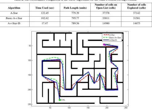
9.6 APPLICATION 1: Solving a Maze Problem with the A-Star and Basic Star and
A-r-Star Algorithms
Artificial intelligence search algorithms are often used to solve maze problems that are common in tortuous games such as the Pacman Maze Game. Such maze problems are similar, and equivalent in some cases, to pathfinding problems faced by robots operating in maze-like environments such as building floorplans and underground mines, for example. The first application is to use the three pathfinder algorithms to solve a simple 256 x 256 maze problem. Figure 12 shows the maze and respective paths found between the indicated start and goal nodes. The performances of the algorithms are summarized in Table 2. Here, the path length is measure using
[image:10.595.74.270.331.474.2]the Euclidean distance. Note that the paths returned by and have bulges that make the path suboptimal. These bulges can be eliminated using the techniques proposed in Section 9, as shown in Figure 6.
Table 2. The Performance Comparison of the Three Algorithms for the Maze Problem Solving Problem
Algorithm Time Used (sec) Path Length (units)
Number of cells on Open List (cells)
Number of cells Explored (cells)
A-Star 122.45 779.39 37378 37142
Basic-A-r-Star 102.62 795.77 33011 31581
A-r-Star-IS 17.47 789.56 14980 14675
Figure 12: How , and operating on a uniform grid world solves a maze problem
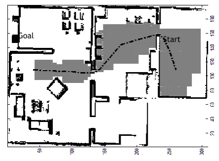
9.7 APPLICATION 2: Path planning in a Simulated Home using A-r-Star Pathfinder
(a) The Webots Prototype of the home environment
(b) A binary occupancy grid map of the environment showing the path (center line), the obstacle zone (black nodes), the skip zones (gray
[image:12.595.323.545.101.264.2]nodes) and the obstacle-free zone (white nodes). Figure 13: Path planning in a prototype home environment using the pathfinder
10
CONCLUSION AND FUTURE WORK
This paper presents a new pathfinder called for offline path planning that outperforms the pathfinder in a uniform gridded sparse world. It also presents various demonstrations of some of the desirable properties of this algorithm and provesthat the performance of this new algorithm matches that of the pathfinder running on a quadtree decomposed world. More research is being performed to extend the algorithm to operate on non-binary grid worlds and to develop an incremental version of this algorithm, and the results will be compared with the performance of the incremental pathfinders ( and its variants.
11
ACKNOWLEDGMENT
This material is based in part upon work supported by the National Science Foundation (NSF) under Cooperative Agreement No. DBI-0939454. Any opinions, findings and conclusions are those of the author(s) and do not necessarily reflect the views of the National Science Foundation.
12
REFERENCES
[1] Cikes, M., Dakulovic, M., and Petrovic, I. 2011. The path planning algorithms for a mobile robot based on the occupancy grid map of the environment; A comparative study.In Proceedings of the XXIII International Symposium on Information, Communication and Automation Technologies, 1-8.
[2] Hart, P. E., Nilsson, N. J., and Raphael, B. 1968. A formal basis for the heuristic determination of minimum cost paths.IEEE Transactions on Systems Science and Cybernetics 4 (2), 100-107.
[3] Dechter, R. and Pearl, J. 1985. Generalized best-first search strategies and the optimality of A*. J. ACM 32 (3), 505-536.
[4] Kambhampati, S. and Davis, L. S. 1986. Multiresolution path planning for mobile robots.IEEE Journal of Robotics and Automation 2 (3) (Sep 1986), 135-145.
[5] Verwer, B. J. H. 1990. A multiresolution work space, multiresolution configuration space approach to solve the path planning problem.In Proceedings of the IEEE International Conference on Robotics and Automation 2103, 2107-2112.
[6] Botea, A., Muller, M., and Schaeffer, J. 2004. Near optimal hierarchical path-finding. Computers and Games 3, 33–38.
[7] Fredman, M. L. and Willard, D. E. 1993. Surpassing the information theoretic bound with fusion trees. Journal of Computer and System Sciences 47 (3), 424-436.
[8] Cowlagi, R. V. and Tsiotras, P. 2012. Multi-resolution path planning: theoretical analysis, efficient implementation, and extensions to dynamic environments. In Proceedings of the49th IEEE Conference on Decision and Control. 1384-1390.
[9] Daniel, K., Nash, A., Koenig, S., and Felner, A. 2010. “Theta*: any-angle path planning on grids. Journal of Artificial Intelligence Research 39, 533-579.
[10] Stentz, A. 1995. Optimal and efficient path planning for unknown and dynamic environments. International Journal of Robotics & Automation 10 (3), 89-100.
[11] Stentz, A. 1994. Optimal and efficient path planning for partially-known environments.In Proceedings of the IEEE International Conference on Robotics and Automation 3314, 3310-3317.
[12] Stentz, A. 1995. The Focussed D* algorithm for real-time replanning.In Proceedings of the International Joint Conference on Artificial Intelligence.
[13] Koenig, S. and Likhachev, M. 2002. D*lite.In Proceedings of the Eighteenth National Conference on Artificial Intelligence, Edmonton, Alberta, Canada, 476-483.
[14] Ferguson, D. and Stentz, A. 2007. Field D*: an interpolation-based path planner and replanner. In Thrun,
Kitchen
Living room
Bed Room
FitnessRoo m
WashRoom
Goal Start
S., Brooks, R. and Durrant-Whyte, H., eds., Robotics Research. Springer Tracts in Advanced Robotics,Springer Berlin Heidelberg, 239-253.
[15] Carsten, J., Ferguson, D., and Stentz, A. 2006. 3D Field D: improved path planning and replanning in three dimensions.In Proceedings of the IEEE/RSJ International Conference on Intelligent Robots and Systems. 3381-3386.
[16] Shih-Ying, C., Tsui-Ping, C., and Zhi-Hong, C. 2012. An efficient theta-join query processing algorithm on MapReduce framework.In Proceedings of the International Symposium on Computer, Consumer and Control . 686-689.
[17] Aizawa, K. and Tanaka, S. 2009. A constant-time algorithm for finding neighbors in quadtrees.IEEE Transactions on Pattern Analysis and Machine Intelligence 31 (7), 1178-1183.
[18] Schroeder, W. J., Zarge, J. A., and Lorensen, W. E. 1992. Decimation of triangle meshes. SIGGRAPH Comput. Graph. 26(2), 65-70.
[19] Huang, C. T. and Mitchell, O. R. 1994. A Euclidean distance transform using grayscale morphology decomposition.IEEE Transactions on Pattern Analysis and Machine Intelligence 16 (4), 443-448.
[20] Chung, K.-L., Huang, H.-L., and Lu, H.-I. 2004. Efficient region segmentation on compressed gray images using quadtree and shading representation. Pattern Recognition 37 (8), 1591-1605.