Neural Networks A General Framework for Non Linear Function Approximation

Neural Networks. A General Framework

for Non-Linear Function Approximation

Fischer, Manfred M.

Vienna University of Economics and Business

2006

Online at

https://mpra.ub.uni-muenchen.de/77776/

Version 1 - 20-04-2006

Neural Networks

A General Framework for Non-Linear Function

Approximation

MANFRED M. FISCHER

Institute for Economic Geography and GIScience Vienna University of Economics and Business Administration

1 Introduction

noise, diversity and dimensionality of typical data sets make formal problem specification difficult.

This contribution is intended as a convenient resource for GIScholars interested in a more fundamental view of the neural network modelling approach. We discuss some important issues that are central for successful application development. But it would be impossible to provide a comprehensive treatment and to consider all the different neural network models in a single paper. We limit the scope to feedforward neural networks, the leading example of neural networks. Feedforward network models have a lot to offer and we use appropriate statistical arguments to gain important insights into the problems and properties of this network approach.

The paper is organized as follows. The next section continues to provide the context in which neural network modelling is considered by introducing relevant concepts of probability fundamental for this type of modelling. Neural networks, of the kind considered here, can be viewed as a very general framework for non-linear function approximation where the form of the mapping is governed by a number of adjustable parameters. For example, in the case of regression problems, it is the regression function that we wish to approximate. The network inputs are the explanatory variables, and the weights the regression parameters.

Neural networks that have a single hidden layer architecture with N

input nodes and a single output are described in some detail in Section 3. They represent a rich and flexible class of universal approximators. Section 4 discusses the notion of network performance and shows a way how to choose the best approximation and, moreover, formalizes the requirement that a network model shows good generalization (out-of-sample) performance.

Neural Networks 3

search and global search. The latter is expected to allow the network to escape from local minima during learning.

Motivated by the desire to obtain distributional results for the approximation that rely neither on large scale sample size nor on artificial data-generating assumptions, Section 6 shows how bootstrapping pairs estimation provides an unconditional bootstrap distribution and can give trustworthy estimates even if the model is wrong. One of the most important factors in the success of a practical application of neural networks is the search for an appropriate technique for determining network complexity. Section 7 addresses this issue and provides insights into current best practice to optimize complexity so to perform well on generalization tasks.

Section 8 discusses the standard approach for assessing the generalization (out-of-sample) performance of a neural network and suggests the use of bootstrapping to overcome the problem of static data splitting. Finally, Section 9 contains some concluding remarks. The references included are intended to provide useful pointers to the literature rather than a complete record of the historical development of the field.

2 Background

To start we must specify the context in which neural network modelling is considered. We assume that a sequence {Zu=(Yu, Xu)} of independent identically distributed (iid) random (N+1)x1 vectors [N∈

฀

interest. In forecasting problems, for example, Yu is a variable that we

wish to forecast on the basis of a set of N variables Xu which may itself

contain past values of Yu.

We take the unknown function of interest to be the conditional expectation of Yu, given Xu, E(Yu | Xu). Whenever E(Yu | Xu) exists and this

is the case for E(Yu)< ∞, it can be represented solely as a function of Xu,

that is g(Xu)=E(Yu | Xu) for some mapping g:ℜ N_→ℜ

Yu can assume a continuum of values, g(Xu) gives the expected value for

Yu given that Xu= xu. We may also write

( )

u u u

Y =g X +ε (1)

where ε_u ≡Y_u−E Y( _u|X_u)is a random error with conditional expectation zero given Xu. When the relationship between Yu and Xu is deterministic,

u

ε is zero given any realization of Xu; otherwise, εuis non-zero with

positive probability (White 1990).

Our problem is to approximate (estimate, learn) the mapping g from a realization of the sequence {Zu} or in other words to construct an

estimator ˆg of g from a realization of {Zu}. For this purpose we consider

the output functions of single hidden layer feedforward networks in the section that follows.

Before doing so we should note that in practice we observe a realization of only a finite part of the sequence {Zu}, a training sample of

size U: {zu=(yu, xu): u=1, ..., U}. Because g is an element of a space, say

G, of functions, we have essentially no hope of learning g in any complete sense from a sample of finite size. Nevertheless, it is possible to approximate g to some degree of accuracy using a sample of size U, and to construct increasingly accurate approximations with increasing U

(White 1990).

3 Feedforward Neural Networks

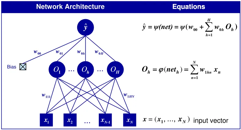
Figure 1 A feedforward network for approximating the unknown mapping g(.):ℜN_→ℜ

where

ˆ ( )

y=y net is the network forecast for the input vector (x1, …, xN),

00 ₁ 0

H h h h

net=w +

∑

outputs of the hidden units calculated as Oh= ϕ(neth) and ₁

1

N h n hn n

net =

∑

ˆ ₀₀

∑

=1 = = ( +

)

y ψ(net) ψ w w

O

Network Architecture Equations Network Architecture Equations

input vector 2 x

y

ˆ

O

O

O

w w0h w0H

1HN w

...

...

...

)

= _{1 N}

x x

, ...,

x

(

)

∑

1 N

hn n

h

net

w

x

O

=

For concreteness and simplicity, we consider single hidden layer neural network models with N input nodes, H hidden nodes and a single output node in this contribution as shown in Figure 1. Given an input vector

x=(x1, …, xN) the output of this kind of network is given by a function

:

H Ν

φ ℜ ×W → .ℜ The weight (parameter) space W is a compact subset of ℜp _{(p integer) such that for each , ( , . ) :}

H

x φ x W →ℜ is continuous

and for each ( , ...,1 ) , ( . , ) :

N p H

w= w w ∈W φ w ℜ →ℜ is measurable.

Network weights are, thus, restricted to lie in a compact set W of finite dimension p where p indicates the total number of weights. This requirement for network output functions is satisfied by

00 0 1

1 1

( , ) ( ( ))

H N

h hn n

h n

H x w w w w x

φ y ϕ

= =

= +

∑

∑

where w=(w w₀, ₁) is the p-dimensional vector of network weights.

0 ( 00, 01,..., 0H)

w = w w w contains the hidden to output weights and

1 ( 10,..., 1H)

w = w w with

w

(

w

, ...,

w

)

denotes the number of input nodes and H the number of hidden nodes. Note that H is an unambiguous descriptor of the dimensionality p of the weight vector: p=(N+2)H+1. The function φis explicitly indexed by H in order to indicate the dependence. ϕ represents a non-linear hidden unit transfer function and y a linear or non-linear output transfer function, both continuously differentiable of order 2 on ℜ.

The hidden transfer function ϕ(.) is characteristically specified as a function belonging to the family

{ (_{x r s t}, , , ),_{x ℜ}N;_{r ℜ},_{s t}, _ℜ { }}_O

Γ = γ γ= ∈ ∈ ∈ − (3)

with

1 ( )x r s(1 expt x)

γ _{= + +} −

. (4)

Neural Networks 7

different types of transfer functions are appropriate for different cases. In regression contexts, for example, linear or quasi-linear output transfer functions are useful, while a generalization of the logistic sigmoid transfer function known as normalized exponential or softmax transfer function is appropriate in the case of classification problems involving mutually exclusive classes.

Models of the form (2) represent a rich and flexible class of approximators. It is now well established that neural networks of the type (2) with linear output and sigmoid hidden layer transfer functions can approximate any continuous function g uniformly on compacta, provided that sufficiently many hidden units are available (Cybenko 1989, Funahashi 1989, Hecht-Nielsen 1989, Hornik et al. 1989). These results establish single hidden layer feedforward network models as a class of universal approximators.

4 Network Performance

If we view (2) as generating a family of approximations – as w ranges over W – to some specific empirical phenomenon relating inputs x to some y, then we need a way to pick a best approximation from this family.

The goodness of an approximation can be evaluated using a performance function, say π, that measures how well the model output given by φ_H( , )x w matches the target y corresponding to given inputs x. The performance ( ,π y φ_H( , ))x w should be zero when target and model output match and positive otherwise. A measure of overall network performance is given by the unconditional expectation of the random quantity ( ,π Y φ_H( , )),X w formally expressed as

( ) ( , ( , )) ( )

[ ( , ( , ))]

u H u

H

L w y x w d z

E Y X w

π φ ν

π φ

=

=

with w∈W and π a suitably chosen function. We call L(w) the expected performance [loss] function of the neural network. It is worth noting that the function depends only on the weights w, and not on particular realizations y and x. These have been averaged out. This averaging is done in the integral representation defining L. The integral is a Lebesque integral taken over RN+1

. The second expression reflects the fact that averaging ( ,π y φ_H( , ))x w over the joint distribution X and Y [that is,ν] provides the mathematical expectation E(.) of the random performance

( ,Y _H( , ))X w

π φ (see White 1989a).

Choosing w to solve min{L(w): w∈W} results in a network model that produces the smallest average performance, given an input randomly drawn from the operating environment. This provides a way to choose the best approximation and formalizes the requirement that the model generalizes well, that is, performs well on an out-of-sample sample (White 1989a).

Because Equation (2) can only approximate the empirical relationship between X and Y, it produces an inherently misspecified model. This implies that the solution arg min{L(w): w∈W}, say w*, depends on the choice of both π and ν. Thus, πhas to be carefully chosen to embody the desired network performance and the target-input pair (y,

x) must be drawn from the true operating environment. Otherwise, w*

indexes a suboptimal network model (White 1989b).

Let us consider learning based on least squares performance, the leading example of learning:

2 ( ,Yu H(X wu, )) (Yu H(X wu, ))

π φ = −φ

.

Least squares learning has the goal to find a solution w* that minimizes the expected performance function L(w):

2

min ( ) min [( _{u H}( _u, )) ]

Neural Networks 9

Note that w* indexes a mean squared error-optimal approximation

φH( . , w

*

) to the unknown function g (White 1989a). In practice, we consider least squares learning over a training set of size U. Let ˆwU

denote the solution to the problem

2 1

1

min ( ) min ( ( , ))

U

U u H u

w w

u

U

L w y φ x w

∈ ∈ ₌

 

=  − 



∑

W W (8)

where L_U( )w is the average least squares performance of the network over the training sample of size U, by construction. The discrepancy between the "best" approximating model ( *)

H x, w

φ and φ_H(x, wˆ_U) expresses the magnitude of the lack of fit due to sampling variation. It depends on the data and the estimation procedure used to solve the optimization problem. In general its expectation increases with the dimensionality of the weight vector. Obviously, it can not be computed, unless the underlying function g(x) is known.

But it can be shown that as the size of the training sample, U, tends to infinity, L_U( )w converges to ( )L w and ˆwUto

*

w . For an analytical proof see White (1989a). Sussmann (1992) and Chen et al. (1993) provide conditions sufficient to ensure uniqueness of w* in a suitable W for specific network configurations.

5 Network Learning Procedures

In the previous section we have seen that the objective of network learning [parameter estimation] is to find w* to minimize ( )L w , given an appropriately chosen neural network. The fact that w* is unknown prevents us from calculating (L w*) directly. But ˆwU consistently

squares regression so that the solution to the problem, ˆwU, is a non-linear

least squares estimator1.

Now consider, how the optimization problem (8) can be solved in real world situations. In general, we look for a global solution to what is characteristically a highly non-linear optimization problem. Computing

ˆ_U

w by means of solving the system of normal equations can be

analytically intractable for non-linear models with more than a few parameters. Thus, iterative procedures are generally used. Two broad types of procedures can be distinguished: Local and global search procedures.

The most prominent local search procedures are gradient descent techniques. These can be thought to transfer the minimization problem (8) into an associated system of first-order ordinary differential equations2 which can be written in compact matrix form (see Cichocki and Unbehauen, 1993) as

( , ) _{w U}( )

dw

w s L w

ds = −µ ∇ (9)

with

1_{, ...,}

T p

dw dw

dw

ds ds ds

 

=  

  (10)

U

w is increasingly downward biased with increasing H. The bias arises because the observations for (X Yu, )u are used in arriving at wˆU.

Neural Networks 11

where ∇_w L_U( )w represents the gradient operator of L_U( )w with respect to the p-dimensional parameter vector w. µ( , )w s denotes a p×p

positive definite symmetric matrix with entries depending on time s and the vector ( )w s .

In order to find the desired vector ˆwU that minimizes the loss

function L_U( )w we need to solve the system of ordinary equations (9)-(10) with initial conditions. The minima of L_U( )w are determined by the following trajectory of the gradient system with

ˆ lim ( ).

s

w w s

→∞

= (11)

But it is important to note that we are concerned only with finding the limit rather than determining a detailed picture of the whole trajectory

( )

w s itself. In order to illustrate that the system of differential equations given by (9)-(10) is stable let us determine the time derivative of the average least squares performance function

[

]

1

( ) ( ) ( ) 0

p

T U U k

w U w U k k

dL L w

L w w,s L w

ds = w s µ

∂ ∂

= = − ∇ ∇ ≤

∂ ∂

∑

under the condition that the matrix (µ w,s) is symmetric and positive definite. Relation (12) guarantees under appropriate regularity conditions that the loss function decreases in time and converges to a stable local minimum as s→ ∞. When dw ds/ =0 then this implies ∇_wL_U( ) 0w =

for the system of differential equations. Thus, the stable point coincides either with the minimum or with the inflection point of LU (see Cichocki

and Unbehauen, 1993).

time evaluation of ( )w s will result in the minimization of ( ( ))L w s as time s goes on. The trajectory ( )w s moves along the direction which has the sharpest rate of decrease and is called the direction of steepest descent.

The discrete-time version of the procedure can be written in vector form as

( 1) ( ) ( ) _{w U}( ( ))

w s+ =w s −η s ∇ L w s (13)

with ( ) 0η s ≥ . The parameter ( )η s is called learning rate and determines the length of the step to be taken in the direction of the gradient of

( ( ))

U

L w s . It is important to note that ( )η s should be bounded in a small range to ensure stability of the algorithm. Note that the sometimes extreme local irregularity ('roughness', 'ruggedness') of the function

( ( ))

U

L w s over W may require the development and use of appropriate modifications of the standard procedure given by Equation (13).

The technique of backpropagation popularized in a paper by Rumelhart, Hinton and Williams (1986) can be used for evaluating the derivatives of the loss function L_U( )w . This technique provides a computationally efficient procedure for evaluating such derivatives that are used to calculate the adjustments to be made to the weights3. It corresponds to a propagation of gradient errors backwards through the network. The reader may consult Bishop (1995) for details concerning the specifics of implementation.

Global Search Procedures. Although computationally efficient, gradient based minimization procedures, such as backpropagation of gradient errors, may lead only to local minima of L_U( )w that happen to be close to the initial search point (0)w . As a consequence, the quality of the final solution of the learning problem is highly dependent on the selection of the initial conditions. Global search procedures are expected

Neural Networks 13

to lead to optimal or 'near-optimal' parameter configurations by allowing the network model to escape from local minima during training. Genetic algorithms and the Alopex procedure [a correlation-based procedure] are attractive candidates4.

The success of global search procedures in finding a global minimum of a given function such as L_U( )w over w ∈ W hinges on the balance between an exploration process, a guidance process and a convergence-inducing process (see Hassoun, 1995). The exploration process gives the search a mechanism for sampling a sufficiently diverse set of parameters

w in W. The Alopex procedure, for example, performs an exploration process that is stochastic in nature. The guidance process is an implicit process that evaluates the relative quality of search points and utilizes correlation guidance to move towards regions of higher quality solutions in the parameter space. Finally, the convergence-inducing process

ensures the convergence of the search to find a fixed solution ˆ .wU The

convergence-inducing process implemented in ALOPEX is realized effectively by a parameter T, called temperature in analogy to the simulated annealing procedure, that is gradually decreased over time. The dynamic interaction among these three processes is responsible for giving the Alopex search procedure its global optimizing character.

Global – as opposed to local – search procedures should be used in learning problems where reaching the global optimum is at premium. The price one pays, however, is increased computational requirements. The intrinsic slowness of such procedures is mainly due to the slow but crucial exploration process. This may motivate the development of a hybrid approach that uses global search to identify regions of the parameter space containing local minima and gradient information to actually find them (Fischer, 2002).

Iterative – no matter whether local or global – procedures need both a starting point and a stopping rule. The starting point is usually taken to be a random set of weights. Some care is needed that they are not taken to

be too large in order to avoid that the sigmoid hidden units start with outputs very near to zero or one. The issue of when to stop learning is important. Many ad hoc rules have been proposed. One which seems popular is to have an independent validation set, and training is stopped when the loss function on the validation set starts to rise. It is also not uncommon to use the test set rather than a validation set as the use of a validation set is viewed wasteful.

6 Bootstrap Estimation

Resampling techniques can be used for estimating standard errors and confidence intervals for the model parameters ˆwU, when {Zu} is a

sequence of iid random variables. The term resampling is used to include bootstrapping, jackknifing, cross-validation and their variants. These are techniques primarily used for non-parametric estimation of statistical error. In contrast to Monte Carlo simulations bootstrapping and jackknifing do not require a priori specification of the data-generating mechanism. The estimates of bootstrapping and cross-validation are asymptotically equivalent. Bootstrapping loosely related to jackknifing is conceptually simpler and more straightforward for the required computations (Efron 1982).

The bootstrap pairs approach5 is an intuitive way to apply the bootstrap notion to neural network models. The basic idea of this approach is to draw a large number, say B, of random samples of size U

with replacement from U {( , ) : 1, ..., }

u u

z = y x u= U , compute ˆw_U for

each of the B bootstrap training samples, and use the resulting empirical distribution of the ˆ*b

U

w as an estimate of the sampling of the distribution of ˆw_U. Implementing the approach involves the following steps (Fischer and Reismann 2002a):

5 _{This approach is called bootstrapping pairs in contrast to residuals}

Neural Networks 15

(i) Use the original sample U {( , ) : 1, ..., }.

u u

z = y x u= U

(ii) Draw an iid bootstrap sample U*b _{( *b_, *b_{) : 1, ..., }} u u

z = y x u= U of size U

with replacement from the original sample.

(iii) Use this bootstrap sample to compute a new parameter vector ˆ*b U

w by solving (8) with U*b

z replacing U

z :

{

}

ˆ*b arg min ( *b) : *b p

U U

w = L w w ∈W ⊆ℜ (14)

where p is the number of parameters. ( *b)

U

L w is the average least squares performance of the network over the bootstrap sample of size

U given by

* 2 1 2 1 ( ) ( ( , )) . U

*b b *b *b u H u U

u

L w y φ x w

=

=

∑

(iv) Replicate step (ii)-(iii) many times, say B=100 or B=1,000.

(v) Take the bootstrap parameter estimates ˆ*b U

w (b=1, ..., B) to estimate the standard derivation [the root mean squared error] of the estimation as follows

1 2

* * 2

1 1

1

ˆ (ˆ ˆ ( ))

B b B B U U

b

w w

σ _{− °}

=

 

=_ − _



∑

where

* 1 *

1

ˆ ( ) ˆ .

B b U B U

b=

w _° =

∑

'true' value of the parameter estimate where ˆ ( )wU α and ˆ (1wU −α)

are the 100α and 100(1-α) percentiles of the bootstrap estimation,

B U

Ξ , of ˆ*b U

w (b=1, ..., B).

The rationale underlying the bootstrap approach is simple. We want an estimate of the accuracy of ˆwUand like to use σ σ Θ= ( ) where ( )σ . is

some agreed upon functional that measures accuracy. Θ is the true probability distribution giving rise to the sample {( ,Y_u X_u) :u=1, ..., }U . We do not know Θ, so instead we estimate ˆσB =σ Ξ( UΒ).

Β

U

Ξ is supposed to describe closely the empirical cumulative distribution function ˆΘU, in other words ˆ ( ˆ )

B B U

σ ≈σ Θ . Asymptotically, this means

that as U tends to infinity, the estimate ˆσB tends to ( ˆ ) B U

σ Θ . But for finite samples there will be deviations in general.

7 Network Complexity

In the preceding sections we have considered learning procedures for feedforward neural networks of fixed complexity [that is, H suitably chosen]. Despite the great flexibility which such models can afford in their ability to approximate arbitrary mappings, they are nevertheless fundamentally limited. In particular, feedforward networks will provide only partial approximations to arbitrary mappings g. This performance can be quite poor. A network model, for example, that is too complex (relative to the sample size U) learns too much, but generally performs poorly on generalization tasks, while a network that is too simple will have a large bias and smooth out some of the underlying structure in the data. This highlights the need to appropriately select the complexity of the model in order to achieve the best generalization (out-of-sample) performance (Bishop 1995).

Neural Networks 17

the number of hidden units for a training set of given size as a process consisting of a series of steps that are performed independently:

(i) The first step consists of choosing a specific parametric

representation that is oversized in comparison to the size of the training set used.

(ii) Then in the second step either a performance function such as

LU(w) [possibly including a regularization term

6

] is chosen directly, or in a Bayesian setting, prior distribution on the elements of the data-generation process (noise, model parameter, regularizer, etc.) are specified from which a performance function is derived.

(iii) Utilizing the performance function specified in (ii), the training process is started and continued until a convergence criterion is satisfied. The resulting parametrization of the given model architecture is then placed in a pool of model candidates from which the final model will be chosen.

(iv) To avoid overfitting, model complexity has to be limited. Thus, the next step usually consists of modifying the network model architecture [for example, by pruning weights] or the penalty term [for example, by changing its weighting in the performance function] or the Bayesian prior distributions. The last two modifications then lead to a modification of the performance function. This establishes a new framework for the training process that is then restarted and continued until convergence, yielding another model for the pool.

6 _{In this case in Equation (8) is modified by replacing L}

U(w) through

2 ( )

U

This process is iterated until the pool is assumed to contain a reasonable diversity of the model candidates that are then compared with each other. The model with the best performance on a test set is selected. The methods employed for training may be very sophisticated, while the choice and modification of the network model architecture and performance function is generally ad hoc, or directed by a search heuristic in practice.

Finally note that a heuristic reason why feedforward networks of type (2) might work well with modest numbers of hidden units in real world application domains is that the hidden layer allows a projection onto a subsequence of RN

of much lower dimensionality, within which the approximation can be carried out. In this aspect feedforward neural network models share many of the properties of projection pursuit regression.

8 Assessing the Generalization Performance

The standard approach for assessing the generalization (out-of-sample) performance of a neural network is data splitting. This method simulates learning [training] and generalization by partitioning the data set into three data sets: a training set, a validation set and a testing set. The training set is used for parameter estimation only. The validation set for determining the stopping point before overfitting occurs and for selecting architectural parameters such as H. The generalization performance of the model is tested on the test set using an appropriate performance criterion such as described in Section 5. Note that the validation set must be different from the test set for the assessed performance to be valid.

Neural Networks 19

splitting the data into three disjoint data sets with the power of a resampling technique and allows us to get a better statistical picture of the generalization performance of the model.

The idea behind this approach is to generate B pseudo-replicates of the training sets _zU *b1 _{, validation sets z}U *b2 _{and testing sets z}U *b3 _{, then to} estimate resampled weights ˆ*b

U

w on each training bootstrap sample _zU *b1 as described in the previous section, to stop training on the basis of the associated validation set _zU *b2 _{and to test out-of-sample performance on} the test bootstrap sample _zU *b3 _{. In this bootstrap world, the empirical} bootstrap distribution of the performance measure can be estimated, pseudo-errors can be computed, and used to approximate the distribution of the real errors. The approach is appealing, but characterized by very demanding computational intensity in real world contexts (see Fischer and Reismann 2002b for an application).

9 Concluding Remarks

crucial importance for the success of real world neural network applications.

Neural network modelling will gain further acceptance in GIScience, as its usefulness becomes apparent in a diversity of application domains. There is no doubt in mind that neural network modelling may satisfy two roles in GIScience: as a statistical device to identify relationships in large and complex spatial data sets, and as a way to come to grips with unclear or fuzzy data. In the first instance, neural networks are gaining acceptance as spatial interaction approximators and as classifiers of remotely sensed pixel data; and in the second instance, data that in past years have been disregarded because of their inconclusive nature are being evaluated using neural modelling approaches. This trend is likely to continue, given the mountains of data now being amassed, but also because the methods are tied directly to the new technology that allows for computationally intensive analysis.

References

Bishop, M. (1995). Neural Networks for Pattern Recognition. Oxford University Press, Oxford.

Chen, A.M., Lu, H.M. and Hecht-Nielsen, R. (1993). On the geometry of feedforward neural-network error surfaces. Neural Computation, Vol. 5, 910-926.

Cichocki, A. and Unbehauen, R. (1993). Neural Networks for

Optimization and Signal Processing. John Wiley, Chichester.

Coetzee, F.M. and Stonick, V.L. (1995). Topology and geometry of single hidden layer network. Neural Computation, Vol. 7, 672-705. Cybenko, G. (1989). Approximation by superpositions of a sigmoidal

function. Mathematics of Control Signals and Systems, Vol. 2, 303-314.

Efron, B. (1982). The Jackknife, the Bootstrap and Other Resampling Plans. Society for Industrial and Applied Mathematics, Philadelphia. Efron, B. and Tibshirani, R. (1983). An Introduction to the Bootstrap.

Chapman and Hall, New York.

Neural Networks 21

Fischer, M.M. (2001). Spatial analysis in geography, in: Smelser, N.J. and Baltes, P.B. (Eds.), International Encyclopedia of the Social and Behavioral Sciences, Vol. 22. Elsevier, Oxford, pp. 14752-14758. Fischer, M.M. (2000). Methodological challenges in neural spatial

interaction modelling: The issue of model selection, in: Reggiani, A. (Ed.), Spatial Economic Science: New Frontiers in Theory and Methodology. Springer, Berlin, Heidelberg and New York, pp. 89-101.

Fischer, M.M. and Getis A. (Eds.) (1997). Recent Developments in Spatial Analysis. Spatial Statistics, Behavioural Modelling and Computational Intelligence. Springer, Berlin, Heidelberg and New York.

Fischer, M.M. and Gopal, S. (1994). Artificial neural networks: A new approach to modelling interregional telecommunication flows.

Journal of Regional Science, Vol. 34(4), 503-527.

Fischer, M.M. and Leung, Y. (Eds.) (2001). GeoComputational

Modelling: Techniques and Applications. Springer, Berlin, Heidelberg and New York.

Fischer, M.M. and Leung, Y. (1998). A genetic-algorithm based evolutionary computational neural network for modelling spatial interaction data. The Annals of Regional Science, Vol. 32(3), 437-458.

Fischer, M.M. and Reismann M. (2002a). Evaluating neural spatial interaction modelling by bootstrapping. Networks and Spatial Economics, Vol. 2(3), 255-268.

Fischer, M.M. and Reismann M. (2002b). A methodology for neural spatial interaction modeling. Geographical Analysis, Vol. 34(2), 207-228.

Fischer, M.M., Hlavackova-Schindler K. and Reismann M. (1999). A global search procedure for parameter estimation in neural spatial interaction modelling. Papers in Regional Science, Vol. 78, 119-134. Funahashi, K. (1989). On the approximate realization of continuous

mappings by neural networks. Neural Networks, Vol. 2, 183-192. Gallant, A.R. and White, H. (1988). A Unified Theory of Estimation and

Inference for Nonlinear Dynamic Models. Basil Blackwell, Oxford. Hassoun, M.H. (1995). Fundamentals of Artificial Neural Networks. MIT

Press, Cambridge [MA] and London, England.

Hornik, K., Stinchcombe, M. and White, H. (1989). Multilayer feedforward networks are universal approximators. Neural Networks, Vol 2., 359-368.

Press, W.H., Teukolsky, S.A., Vetterling, W.T. and Flannery, B.P. (1992).

Numerical Recipes in C: The Art of Scientific Computing. Cambridge University Press, Cambridge.

Ripley, B.D. (1996). Pattern Recognition and Neural Networks. Cambridge University Press, Cambridge.

Rumelhart, D.E., Hinton, G.E. and Williams, R.J. (1986). Learning internal representations by error propagation, in: Rumelhart, D.E., McClelland, J.L. and the PDP Research Group (Eds.), Parallel Distributed Processing: Explorations in the Microstructure of cognition. MIT Press, Cambridge [MA], pp. 318-362.

Sussmann, H.J. (1992). Uniqueness of the weights for minimal feedforward nets with a given input-output map. Neural Networks, Vol. 5, 589-593.

White, H. (1990). Connectionist nonparametric regression: Multilayer

feedforward networks can learn arbitrary mappings. Neural

Networks, Vol. 3, 535-550.

White, H. (1989a). Learning in artificial neural networks: A statistical perspective. Neural Computation, Vol. 1, 425-464.

White, H. (1989b). Some asymptotic results for learning in single hidden

layer feedforward network models. Journal of the American

Statistical Association, Vol. 84, 1008-1013.

White, H. and Racine, J. (2001). Statistical inference, the bootstrap, and neural-network modeling with application to foreign exchange rates.

IEEE Transactions on Neural Networks, 12(4), 657-673.

White, H. and Wooldridge, J. (1991). Some results for sieve estimation with dependent observations, in: Barnett, W., Powell, J. and Tauchen, G. (Eds.), Nonparametric and Semiparametric Methods in Econometrics and Statistics. Cambridge University Press, New York.

Zapranis, A. and Refenes, A.-P. (1999). Principles of Neural