Central Upwind Scheme for Solving Multivariate Cell Population Balance Models

http://dx.doi.org/10.4236/am.2014.58110

Central Upwind Scheme for Solving

Multivariate Cell Population

Balance Models

Shahzadi Mubeen ur Rehman, Nadia Kiran, Shamsul Qamar

Department of Mathematics, COMSATS Institute of Information Technology, Islamabad, Pakistan

Email: [email protected]

Received 28 February 2014; revised 28 March 2014; accepted 5 April 2014

Copyright © 2014 by authors and Scientific Research Publishing Inc.

This work is licensed under the Creative Commons Attribution International License (CC BY).

http://creativecommons.org/licenses/by/4.0/

Abstract

Microbial cultures are comprised of heterogeneous cells that differ according to their size and intracellular concentrations of DNA, proteins and other constituents. Because of the included level of details, multi-variable cell population balance models (PBMs) offer the most general way to de-scribe the complicated phenomena associated with cell growth, substrate consumption and prod-uct formation. For that reason, solving and understanding of such models are essential to predict and control cell growth in the processes of biotechnological interest. Such models typically consist of a partial integro-differential equation for describing cell growth and an ordinary integro-diffe- rential equation for representing substrate consumption. However, the involved mathematical complexities make their numerical solutions challenging for the given numerical scheme. In this article, the central upwind scheme is applied to solve the single-variate and bivariate cell popula- tion balance models considering equal and unequal partitioning of cellular materials. The validity of the developed algorithms is verified through several case studies. It was found that the sug-gested scheme is more reliable and effective.

Keywords

Cell Population Balance, Cell Growth, Substrate Consumption, Central Upwind Scheme, Equal and Unequal Partitioning of Cells

1. Introduction

certain size (approximately double to its original size) and then divides into two identical daughter cells. Basi-cally cell division is an exponential process, the two daughter cells further divide into four daughter cells, then four into eight and so on [2]. The environmental factors such as oxygen, pH, temperature and substrate concen-tration greatly affect the cell growth rate. At any point in time t, in heterogeneous population different cells exist at different stages of the cell cycle. The different cells could be differentiated according to their size, DNA and RNA contents, protein contents and other inter-cellular properties. Thus, the developments of accurate mathe-matical models are needed that account for heterogeneities present at the single-cell level.

Various mathematical models exist in the literature for describing dynamics of biological systems. These models consider the cell population as a “continuum” or lumped biophase, thus assuming that it behaves as a homogeneous entity. Cell population balance models (PBMs) are the only models that take into account the fact that cell properties are distributed among the cells of a population, such as protein content, DNA content, etc. Moreover, they have capability to effectively describe the internal chemical structure of the single cell by in-corporating intracellular chemical reactions involving multiple chemical species. Therefore, these models pro-vide the most accurate way of describing the complicated phenomena associated with cell growth, nutrient up-take and/or product formation in microbial populations. They typically consist of multidimensional integrto-par- tial differential equations for describing the dynamics of the state distribution function, nonlinearly coupled with integro-ordinary differential equations accounting for substrate consumption and (or) product formation. Be-cause of their obvious mathematical complexity, the numerical solutions of such models are challenging for the given numerical scheme. In mid 1960s, these models were used for the first time to simulate cell dynamics [3] [4]. Cell PBMs are either single-variable or multi-variable, depending on numbers of variables involved in the system. Multivariable models explain the complicated phenomena of cell development, product formation and substrate consumption as compared to the single-variable models. Despite of these details, bioreactor PBMs are associated with many difficulties. Firstly, for majority cell system the growth rate function, the cell division rate and the partitioning probability density function are not known, that can be overcome by flow cytometry analy-sis. The on-line flow cytometry, when combined with suitable cell population models, develops the computer- based system that provides control of cellular distribution. Secondly, a great computational cost is required to numerically solve multi-variable cell PBMs.

Initially, Hulburt and Katz [5] introduced population balance models in chemical engineering, and these mod-els were later on developed by Randolph and Lason [6]. By the time, their applied nature recognized them to be the vital part of research. The large computational time and unavailability of exact solution were the primary ob-stacles in the development of these balances. The analytical solutions are possible in simplified situations only. Thus, researchers started to find its numerical solution instead of the exact solution. A large number of numeri-cal techniques are present for approximating population balance equations (PBEs) in cheminumeri-cal and biologinumeri-cal engineering, such as the weighted residual method [7], the Monte Carto simulation [8], the method of moments

[9] [10], the finite difference method [11]-[13], the spectral methods [14], the finite element method [15] [16], and the high resolution finite volume scheme [17] [18], etc.

In this article, the high-resolution non-oscillatory central-upwind scheme is applied to solve the single-variate and bivariate cell population balance models considering the equal and unequal partitioning of mother cells [19] [20]. The basic idea of such schemes is that they use information of local propagation speeds and the approx-imated solution is obtained as cell averages. Further, such schemes have an upwind nature, as they take care of directions of wave propagation by measuring the one-sided local speeds. Several case studies are carried out and the results of central-upwind scheme are compared with those obtained from the first order upwind scheme.

2. Single-Variate Cell Population Balance Model

A single-variate cell population balance model that expresses the ratio of nutrients is considered in this section. Let N x t

( )

, is a function that represents the state of entire population with the amount of biomass x at time t

between x and x+dx. The zero moment N0

( )

t and the first moment N t1

( )

respectively describe the total number of cells per unit bio-volume and concentration. They are defined as [13]

( )

max

( )

,min

0 , d ,

d x

x

N t =

∫

N x t x (1)

( )

max

( )

,min

1 , d ,

d x

x

The number density function is defined as

( )

( )

_{( )}

0

,

, N x t .

n x t

N t

= (3)

The computational domain is taken to be xd,min,xmax, where xd,min and xmax represent the minimum and

maximum values for the amount of biomass components of daughter cells, respectively. Let xp,min is smallest value of the mass components of parent cells, where xd,min <xp,min. Moreover, the minimum and maximum values of all mass components are considered to be xd,min =xp,min =0 and xmax=1. Here, c indicates the

growth rate, q x s

( )

, represents the nutrient consumption process, Γ

( )

x s, represents division rate of a cell and D denotes the dilution rate. The partitioning function P x y s

(

, ,

)

illustrates the cellular division process of a parent into daughter cell. It gives the probability that a parent cell having state x gives birth to a daughter cell with state y. The following relation satisfies the normalization condition.

(

)

max ,min

, , d 1.

d x

x P x y s x=

∫

(4)

This means that the amount of biochemical components is conserved at cell partitioning. Particularly, daugh-ter cells cannot have larger amounts of biochemical components than the parent cells. Thus, the probability den-sity function P x y s

(

, ,

)

must be zero for all states of daughter cells which are larger than the states of parent cells,

(

, ,

)

0, for .

P x y s = x>y (5)

Furthermore, the probability of a dividing cell with physiological state y to produce a daughter cell of state x must be equal to the probability of producing a daughter cell of state y−x, i.e.

(

, ,

)

(

, ,

)

.

P x y s =P y−x y s (6)

Due to the above-mentioned hypothesis and process description, the dynamics of the state distribution func-tion N x t

( )

, is described by the general cell population balance equation [13]

( )

,

(

( ) ( )

, ,

)

_{( )}

, ,

g x s N x t N x t

Q x t

t x

∂ ∂

+ =

∂ ∂ (7)

where

( )

( ) ( )

( )

max

( ) ( ) (

)

, Γ , , , 2 x Γ , , , , d ,

x

Q x t = − x s N x t −DN x t +

∫

y s N y t P x y s x (8) with initial conditions

( )

, 0 0

( )

.

N x =N x (9)

Let us define boundary b of the state as a point where at least one quantity of biochemical components obtains either its minimum value or its maximum value. Then, the boundary conditions are given as

( ) ( )

, , 0, .

g x s N x t = ∀ ∈x b (10)

Equation (8) has three terms, the first term shows accumulation, the second term accounts for the growth into larger cells, and the third term is the source term. In the source term (c.f. Equation (8)), the first term represents loss of cells due to the partitioning of cells which leads to the birth of daughter cells. The second term is the di-lution rate. The integral birth term is multiplied by the factor 2 for representing the division of a parent cell into two daughter cells. The equal partitioning, where each mass of a mother cell is equally divided into two daugh-ter cells, can be mathematically described by replacing the partition probability density function by a Dirac delta function

(

, ,

)

.

2

y P x y s =δ _x− _

  (11)

( )

( ) ( )

( )

2

(

) (

)

, Γ , , , 2 Γ 2 , 2 , .

Q x t = − x s N x t −DN x t + x s N x t (12)

Thus, the integral term disappears. Since the maximum and minimum values of the dividing cell are xp,min and xp,max, respectively, the corresponding values for each newborn cell must be xd,min=xp,min 2 and xmax=

,max 2

p

x , respectively. Thus, the birth term in Equation (12) exists only for the domain x∈ xp,min 2 ,xp,max 2. The substrate consumption in time is described by an ordinary integro-differential equation of the form [13]

(

)

max

( ) ( )

,min

d

, , d ,

d d

x

f _x

s

D s s N x t q x s x

t = − −

∫

(13)

with initial conditions

( )

0 0

s =s . (14)

The first term in Equation (13) denotes the inlet minus outlet rates from the reactor, and the integral term de-scribes the rate of loss of substrate due to cell growth. Here, q x s

( )

, denotes the consumption rate and s_f is the saturation concentration. In this model, coupling is the only reason for nonlinearity. For a constant abiotic environment, the problem becomes linear.

3. Numerical Scheme for Single-Variate Cell PBM

Here, the semi discrete central-upwind scheme is derived to numerically approximate the PBE model in Equa-tion (7) [19] [20]. Before applying the scheme, we need to discretize the computational domain. Let n be the

number of discretization points and 1 2

for 1, , 1

i

x i n

−

 

= +

 

 

   are partitions of the given interval xd,min,xmax.

Moreover, ∆x denotes the constant width of each grid interval, xi represent the cell centers, and 1 2 i x

±

indi-cate the cell boundaries. We refer,

1 1 max 1

2 2 2

0, , . , for 1, 2, ,

n i

x x x x i x i n

+ +

= = = ∆ = _ . (15)

Moreover,

(

)

max

1 2 1 2 2 and 1 2 1 2 .

1

i i i i i

x

x x x x x x

n

− + + −

= + ∆ = − =

+ (16)

Let Ω = _i: x_{i−1 2},x_{i+1 2}_ for i≥1. For every Ωi, the averaged values of the conservative variables N x t

( )

, and Q x t

( )

, are defined as

( )

1

( )

1

( )

, d and , d

:

i i i

N N t N x t x Q Q x t x

x x

= =

∆ ∆

= . (17)

After integrating Equation (7) over the interval Ω = i xi−1 2,xi+1 2, we get

( )

( )

1 1

2 2

d d

i i

i

i

S t S t

N

Q

t x

+ + −

= − +

∆ . (18)

The numerical fluxes are given as [19]

1 1 1

2 2 2

1 1 1

2 2 2

.

2 2

i i i

i i i

g N g N a

S N N

+ −

+ + + _{+ −}

+ + +

   

+

   

    _{ }

   

= − _ + _

  (19)

Here, N+ and N− shows the piecewise linear reconstruction N for N, namely

1 1 1 1 1

2 2

,

2 2 .

x x

i i i i

i i

x x

N+ N₊ N₊ N− N₊ N

+ +

∆ ∆

Here, x i

N are the first order approximations of N_x

( )

x t_i, and are calculated using a nonlinear limiter that confirms the non-oscillatory nature of reconstruction [19] [20]. The computation of these slopes is given by family of discrete derivatives parameterized with 1≤θ≤2, for example

1 1 1 1

2 2 2 2

, ,

2 x

i

i i i i

N MM θ N θ N N θ N

+ + − −

   

= _ ∆ _∆ + ∆ _ ∆ _

 

 , (21)

where _{1 1}

2

i i

i

N N₊ N

+

∆ = − and

{

1 2

}

{ }

{ }

min if 0, ,

, , max if 0, ,

0 otherwise.

i i i

i i i

x x i

MM x x x x i

 > ∀



=_ < ∀

 

 (22)

Here, ∆ denotes central differencing and MM is the min-mod nonlinear limiter. Further, the local one sided speed at ₁

2 i x

+ is given as [19]

( )

( )

1 1

2 2

max ,

i i

a t g x t t

+ +

  

= _ _ __

 

 . (23)

The second order TVD Runge-Kutta scheme is used to solve Equation (18) to achieve second order accuracy in time. That upgrades N in the following two stages

( )1 n

( )

n

N =N +tL N , (24)

( )

( )

( )

(

1 1

)

1 1

2

n n

N + = N +N + ∆tL N . (25)

where, L N

( )

represent right hand sight of Equation (18) and n

N represents solution at next time step n1 t +

and ∆t is time steps.

4. Bivariate Cell Population Balance Model

This section considers the bivariate cell population balance model for equal partitioning. Here, two property coordinates are used. The evolution of N x y t

(

, ,

)

≥0 is expressed as [13]

(

, ,

)

(

1

( ) (

, , ,

)

)

(

2

( ) (

, , ,

)

)

₍

₎

, ,

g x s N x y t g x s N x y t N x y t

Q x y t

t x y

∂ ∂

∂

+ + =

∂ ∂ ∂ , (26)

where

(

)

(

) ( )

(

)

3

(

) (

)

, , Γ , , , , , 2 Γ 2 ,2 , 2 , 2 , .

Q x y t = − x y s N x t −DN x y t + x y s N x y t (27)

The initial condition is given as

(

)

( ) (

)

3 0

, , 0 , , , ,

N x y =N x y ∀ x y t ∈ . (28)

Here, :=

[

0,∞

)

, N0

( )

x y, ∈2, and the boundary conditions are defined as

(

, ,

) (

, ,

)

0,

(

, ,

)

.

g x y s N x y t = ∀ x y t ∈b (29)

The above cell population balance model is coupled with the mass balance of substrates [13]

(

)

max max

(

) (

)

,min ,min

d

, , , , d d ,

d d d

x x

f _{x x}

s

D s s N x y t q x y s x y

t = − −

∫

∫

(30)

with initial condition

( )

0, 0 0

(

,

)

5. Numerical Scheme for Bivariate Cell PBM

Let nx and ny represents large integers in the x and y-directions, respectively. We assume a Cartesian grid with a

rectangular domain xd,min,xmax  × yd,min,ymax which is concealed by cells 1 1 1 1

2 2 2 2

, ,

ij

i i i i

C x x y y

− + − +

   

=  × 

   

for 1≤ ≤i nx and 1≤ ≤j ny. We take

( )

12 12 12 12

1 1

2 2

, 0, 0 , ,

2 2

i i j j

i j

x x y y

x y x y

− + + − + +

 

= = =

 

 

  . (32)

1 1 1 1

2 2 2 2

,

i j

i i j j

x x x y y y

+ − − + − −

∆ = ∆ = . (33)

At any time t, the cell averaged values N_{i j,}

( )

t for conserved variables are given as

(

)

, ,

1

: 2 , , d d

i j i j

i j

N N N x y t y x

x y

= =

∆ ∆ , (34)

and

(

)

,

1

, , d d i j

Q Q x y t y x

x y

=

∆ ∆ . (35)

The piecewise linear interpolation is described as [19] [20]

(

)

(

,

( )

(

)

( ) (

)

)

,

, ,

,

, , i j x i y j i j

i j i j

i j

N x y t =

∑

N + N x−x + N y−y x , (36)

where, , 1 1 1 1

2 2 2 2

, ,

i j

i i i i

x x x y y

− + − +

   

=  × 

    and

( )

,

x

i j

N and

( )

,

y

i j

N are the approximations of the x and y-de-

rivatives of N at the cell centres

(

x y_i, _j

)

. To calculate these partial derivatives, we use the minmod limiter (MM) with 1≤ ≤θ 2,

( )

(

1, ,

) (

1, 1,

) (

, 1,

)

, , ₂ , ,

n i j i j i j i j i j i j

x i j

N N N N N N

N MM

x x x

θ + θ + − θ −

 − − −    =  ∆ ∆ ∆    (37)

( )

(

, 1 ,

) (

, 1 , 1

) (

, , 1

)

, , ₂ , .

n i j i j i j i j i j i j

y

i j

N N N N N N

N MM

y y y

θ + θ + − θ −

 − − −    =  ∆ ∆ ∆    (38)

On integrating Equation (26) over the control volume Ci j, the two dimensional scheme can be expressed as

[19] [20]

1 1 1 1

, , , ,

, 2 2 2 2

,

d

. d

x x y y

i j i j i j i j

i j

i j

S S S S

N

Q

t x y

+ − − + − −

= − − +

∆ ∆ (39)

Here

1 1

1_, 1_, 1

,

2 2 2

1 1 1

, , ,

2 2 2

,

2 2

x

i j i j i j

x

i j i j i j

g N g N a

S N N

− + + + + _{− +} + + +     +         _{ }     = + _ − _

  (40)

2 2

1 1 1

, , ,

2 2 2

1 1 1

, , ,

2 2 2

,

2 2

x

i j i j i j

x

i j i j i j

g N g N a

S N N

− + + + + − + + + +     +         _{ }     = + _ − _

where, we have

( )

( )

1 , 1 1,

, 1,

, ,

2 2

,

2 2

x x

i j i j

i j i j

i j i j

x x

N− N N N+ N₊ N

+

+ +

∆ ∆

= + = − , (42)

( )

( )

1 , _, 1 , 1 _{, 1}

, ,

2 2

, .

2 2

y y

i j _{i j} i j _{i j}

i j i j

y y

N− N N N+ N ₊ N

+

+ +

∆ ∆

= + = − (43)

The local speeds are computed as

1

1 1

, ,

2 2

, x

i j i j

a ρ g N±

+ +

  

= _ _ __

 

  (44)

12

1 1

, ,

2 2

. y

i j i j

a ρ g N±

+ +

  

= _ _ __

 

  (45)

6. Numerical Case Studies

In this section, a few single-variate and bivariate case studies are considered. The suggested numerical schemes are qualitatively and quantitatively analyzed.

6.1. Test Problem 1: Single-Variate Case

The following presumptions are considered for this problem

• The Gaussian division probability density function is taken as the initial distribution.

• The dilution rate D = 0.

• Due to constant abiotic environment, Equation (13) for substrate consumption is not considered.

• Growth rate functions are consider as: 1) Constant growth rate:

( )

0

1, 1 .

d

m g x h h

U

= = (46)

2) Linear growth rate:

( )

1 1

ln 2

, .

d

g x h x h U

= = (47)

3) Quadratic growth rate:

( )

2

1 1

0

1

, .

2 d

g x h x h

m U

= = (48)

where, m0 is average mass at time t and Ud is the average doubling time. In the unequal partitioning, the number

density function does not show a periodic behavior. In that case, the partitioning mechanism is calculated by be-ta distribution [13] [21]

( )

_{( )}

1 1 1 1

, 1

,

r r

x x

P x y

B r r y y y

− −

    

= _{   } − _

     . (49)

The division function is given as [13]

(

)

( )

( )

(

,min

)

( )

, , ,

1 d

p x

x

f x

x y s g x s

f y y

 

 

Γ _{= } 

 − 

 



∫



. (50)

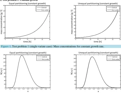
In the case of constant, linear and quadratic growth rates doubling time for equal and unequal partitioning are taken to be Ud = 5h, Ud = 2h and Ud = 5h and simulation times are 30h, 20h and 30h, respectively.Figures 1-4

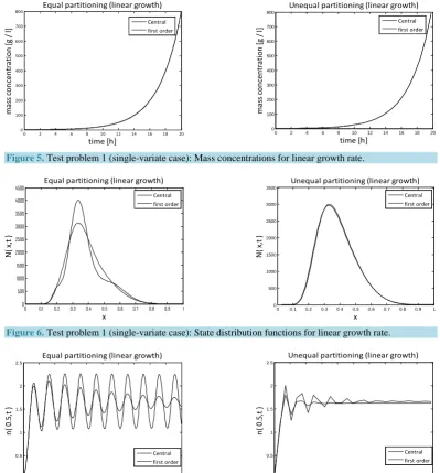
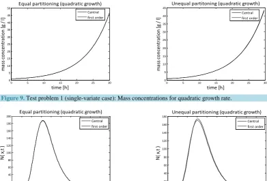
show the constant growths of state distribution function and number density function in two and three dimen-sions obtained by the comparison of upwind central scheme with first order backward difference method. Fig-ures 5-8 describe the linear growth obtained by the same comparison of upwind central scheme with first order backward difference method. Similarly,Figures 9-12 show quadratic growth. The values of parametric are giv-en inTable 1. From the figures, it is clear that in both cases of equal partitioning and unequal partitioning, solu-tion reaches the fastest for quadratic growth and slowest for the linear growth and it is in between in constant growth. It is observed from figure that when time is double the mass concentration become double and also it is obvious from above comparison that first order scheme is more diffusive while central scheme shows accuracy. The results verify that central scheme can be used to capture such profiles more efficiently and accurately.

6.2. Test Problem 2: Single-Variate Case

In this problem, the following assumptions are taken into account. Otherparametric values are listed inTable 2.

In this case growth rates are also depending on the substrate concentration. Therefore, Equations (7) and (13) are solved together.

[image:8.595.90.537.444.713.2]

• The growth rate is taken as [13]-[15]

Table 1. Parametric value for test problem 1 (single-variate case).

Description Symbol Value Units

Doubling time for constant growth Ud 5 h

Doubling time for linear growth Ud 2 h

Doubling time for quadratic growth Ud 5 h

Mean of Gaussian initial condition µ1=µ2 0.2875 -

SD of Gaussian initial condition σ σ1= 2 0.0675 -

Mean of Gaussian division probability density function µ1=µ2 0.575 -

SD of Gaussian division probability density function σ σ1= 2 0.125 -

Parameter for symmetric beta distribution r 40 -

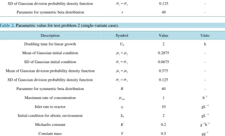
Table 2. Parametric value for test problem 2 (single-variate case).

Description Symbol Value Units

Doubling time for linear growth Ud 2 h

Mean of Gaussian initial condition µ1=µ2 0.2875 -

SD of Gaussian initial condition σ σ1= 2 0.0675 -

Mean of Gaussian division probability density function µ1=µ2 0.575 -

SD of Gaussian division probability density function σ σ1= 2 0.125 -

Parameter for symmetric beta distribution R 40 -

Maximum rate of concentration µmax 1 h

−1

Inlet rate to reactor sf 10 gL−1

Initial condition for abiotic environment S0 2 gL−1

Michaelis constant K 0.2 g−1h−1

1) Test problem 1: Constant growth

[image:9.595.115.508.90.393.2]

Figure 1. Test problem 1 (single-variate case): Mass concentrations for constant growth rate.

[image:9.595.119.506.412.548.2]

Figure 2. Test problem 1 (single-variate case): State distribution functions for constant growth rate.

[image:9.595.117.510.571.707.2]

Figure 3. Test problem 1 (single-variate case): Number density functions for constant growth rate.

Figure 4. Test problem 1 (single-variate case): Number density functions for constant growth rate in 3-D.

0 5 10 15 20 25 30 0

10 20 30 40 50 60

time [h]

m

as

s c

on

ce

nt

rat

io

n [

g /

l]

Equal partitioning (constant growth)

Central first order

0 5 10 15 20 25 30 0

5 10 15 20 25 30 35 40 45 50

time [h]

m

as

s c

on

ce

nt

rat

io

n [

g /

l]

Unequal partitioning (constant growth)

Central first order

0 0.1 0.2 0.3 0.4 0.5 0.6 0.7 0.8 0.9 1 0

20 40 60 80 100 120 140 160 180

x

N

( x,

t )

Equal partitioning (constant growth)

Central first order

0 0.1 0.2 0.3 0.4 0.5 0.6 0.7 0.8 0.9 1 0

20 40 60 80 100 120 140 160 180

x

N

( x,

t )

Unequal partitioning (constant growth)

Central first order

0 5 10 15 20 25 30 0

0.5 1 1.5 2 2.5 3 3.5

time [h]

n(

0.

5,

t )

Equal partitioning (constant growth)

Central first order

0 5 10 15 20 25 30 0

0.5 1 1.5 2 2.5 3 3.5

time [h]

n(

0.

5,

t )

Unequal partitioning (constant growth)

2) Test problem 1: Linear growth

[image:10.595.117.505.95.234.2]

Figure 5. Test problem 1 (single-variate case): Mass concentrations for linear growth rate.

[image:10.595.112.512.96.526.2]

Figure 6. Test problem 1 (single-variate case): State distribution functions for linear growth rate.

[image:10.595.115.512.412.548.2]

Figure 7. Test problem 1 (single-variate case): Number density functions for linear growth rate.

Figure 8. Test problem 1 (single-variate case): Number density functions for linear growth rate in 3-D.

0 2 4 6 8 10 12 14 16 18 20

0 100 200 300 400 500 600 700 800

time [h]

m

as

s c

on

ce

nt

rat

io

n [

g /

l]

Equal partitioning (linear growth)

Central first order

0 2 4 6 8 10 12 14 16 18 20 0

100 200 300 400 500 600 700 800

time [h]

m

as

s c

on

ce

nt

rat

io

n [

g /

l]

Unequal partitioning (linear growth)

Central first order

0 0.1 0.2 0.3 0.4 0.5 0.6 0.7 0.8 0.9 1 0

500 1000 1500 2000 2500 3000 3500 4000 4500

x

N

( x,

t )

Equal partitioning (linear growth)

Central first order

0 0.1 0.2 0.3 0.4 0.5 0.6 0.7 0.8 0.9 1 0

500 1000 1500 2000 2500 3000 3500

x

N

( x,

t )

Unequal partitioning (linear growth)

Central first order

0 2 4 6 8 10 12 14 16 18 20 0

0.5 1 1.5 2 2.5

time [h]

n(

0.

5,

t )

Equal partitioning (linear growth)

Central first order

0 2 4 6 8 10 12 14 16 18 20 0

0.5 1 1.5 2 2.5

time [h]

n(

0.

5,

t )

Unequal partitioning (linear growth)

[image:10.595.116.510.572.708.2]

3) Test problem 1: Quadratic growth

[image:11.595.116.508.96.361.2]

Figure 9. Test problem 1 (single-variate case): Mass concentrations for quadratic growth rate.

[image:11.595.116.511.259.391.2]

Figure 10. Test problem 1 (single-variate case): State distribution function for quadratic growth.

Figure 11. Test problem 1 (single-variate case): Number density function for quadratic growth.

Figure 12. Test problem 1 (single-variate case): Number density functions for quadratic growth in 3-D.

0 5 10 15 20 25 30 0

5 10 15 20 25 30 35 40 45 50

time [h]

m

as

s c

on

ce

nt

rat

io

n [

g /

l]

Equal partitioning (quadratic growth)

Central first order

0 5 10 15 20 25 30 0

5 10 15 20 25 30 35 40 45

time [h]

m

as

s c

on

ce

nt

rat

io

n [

g /

l]

Unequal partitoning (quadratic growth)

Central first order

0 0.1 0.2 0.3 0.4 0.5 0.6 0.7 0.8 0.9 1 0

20 40 60 80 100 120 140 160 180 200

x

N

( x,

t )

Equal partitioning (quadratic growth)

Central first order

0 0.1 0.2 0.3 0.4 0.5 0.6 0.7 0.8 0.9 1 0

20 40 60 80 100 120 140 160 180

x

N

( x,

t )

Unequal partitioning (quadratic growth)

Central first order

0 5 10 15 20 25 30 0

0.2 0.4 0.6 0.8 1 1.2 1.4

time [h]

n(

0.

5,

t )

Equal partitioning (quadratic growth)

Central first order

0 5 10 15 20 25 30 0

0.2 0.4 0.6 0.8 1 1.2 1.4

time [h]

n(

0.

5,

t )

Unequal partitioning (quadratic growth)

[image:11.595.120.508.413.550.2] [image:11.595.116.509.571.707.2]

( )

_, maxs _.

g x s s

K

µ

 

=_ + _

  (51)

where µmax represents the maximum concentration of the substrates and K is the Michaelis constant describing

the substrate concentration due to which the reaction rate is equal to half of µmax.

• The cell consumption rate is given as [13]-[15]

( )

_, maxs 1

q x s s

K y

µ

 

=_ + _

  . (52)

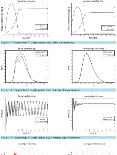
Here y is constant mass. Take doubling time is Ud =2 ,h and the simulation time is 20h.Figures 13-16 dis-play the numerical results for equal and unequal partitioning. The numerical results of the mass concentrations are similar to those available in the literature [13]. In equal partitioning, the number density function represents the constantly oscillatory behavior which disappears in unequal partitioning. From these results it can be noticed that central scheme has comparable accuracy and the first order scheme is diffusive.

6.3. Test Problems 3: Bivariate Case

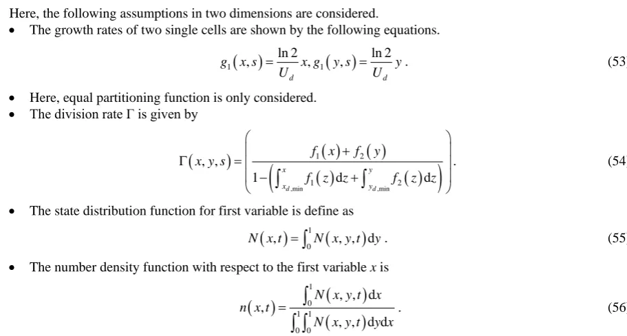
Here, the following assumptions in two dimensions are considered.

• The growth rates of two single cells are shown by the following equations.

( )

( )

1 1

ln 2 ln 2

, , ,

d d

g x s x g y s y

U U

= = . (53)

• Here, equal partitioning function is only considered.

• The division rate Γ is given by

(

)

( )

( )

( )

( )

(

,min ,min

)

1 2

1 2

, ,

1 d d

d d

x y

x y

f x f y x y s

f z z f z z

 

 + 

Γ _{=  }

 − + 



∫

∫



. (54)

• The state distribution function for first variable is define as

( )

1

(

)

0

, , , d

N x t =

∫

N x y t y. (55)

• The number density function with respect to the first variable x is

( )

(

)

(

)

1

0 1 1 0 0

, , d

,

, , d d

N x y t x n x t

N x y t y x

=

∫

[image:12.595.80.536.285.529.2]

∫ ∫

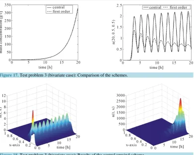
. (56)

Figure 17shows the comparison of mass concentration and middle point of number density function obtained by central upwind and first order schemes. From this figure it is evident that central schemes confine the period-ic behavior of the mid-point of the number density function. The reason, however, is that partitioning density function and growth rates are the same as used in Test problem 1 and mass Equation (13) is not considered be-cause growth rates are independent of substrate concentration s. Due to numerical diffusion in the first order scheme, it is unable to maintain the period oscillations.Figure 18 shows the 2D plots of number density func-tion and state distribufunc-tion funcfunc-tion obtained from the central scheme. By integrating the number density funcfunc-tion and state distribution function with respect to second variable y, we can obtain these results (c.f. Equations (55) and (56)). Thus, the proposed scheme is also accurate in the bivariate case.

7. Conclusion

[image:13.595.114.513.85.612.2]

Figure 13. Test problem 2 (single-variate case): Mass concentrations.

Figure 14. Test problem 2 (single-variate case) State distribution functions.

[image:13.595.115.508.515.699.2]

Figure 15. Test problem 2 (single-variate case): Number density functions.

Figure 16. Test problem 2 (single-variate case): Number density functions in 3-D.

0 2 4 6 8 10 12 14 16 18 20 0

1 2 3 4 5 6

time [h]

m

as

s c

on

ce

nt

rat

io

n [

g /

l]

Equal partitioning

Central first order

0 2 4 6 8 10 12 14 16 18 20 0

1 2 3 4 5 6 7

time [h]

m

as

s c

on

ce

nt

rat

io

n [

g /

l]

unequal partitioning

Central first order

0 0.1 0.2 0.3 0.4 0.5 0.6 0.7 0.8 0.9 1 0

5 10 15 20 25 30 35 40 45 50

x

N

( x,

t )

Equal partitioning

Central first order

0 0.1 0.2 0.3 0.4 0.5 0.6 0.7 0.8 0.9 1 0

5 10 15 20 25 30 35 40 45 50

x

N

( x,

t )

Unequal partitioning

Central first order

0 2 4 6 8 10 12 14 16 18 20 0

0.5 1 1.5 2 2.5

time [h]

n(

0.

5,

t )

Equal partitioning

Central first order

0 2 4 6 8 10 12 14 16 18 20 0

0.2 0.4 0.6 0.8 1 1.2 1.4 1.6 1.8 2

time [h]

n(

0.

5,

t )

Unequal partitioning

[image:14.595.119.511.78.391.2]

Figure 17. Test problem 3 (bivariate case): Comparison of the schemes.

Figure 18. Test problem 3 (bivariate case): Results of the central upwind scheme.

higher order schemes. The numerical test problems verify the usefulness of the suggested-scheme which is computationally efficient, accurate, and easily applicable.

References

[1] Roels, J.A. (1983) Energetics and Kinetics in Biotechnology. Elsevier, Amsterdam.

[2] Slavov, N. and Botstein, D. (2011) Coupling among Growth Rate Response, Metabolic Cycle and Cell Division Cycle in Yeast. Molecular Biology of the Cell, 22, 1997-2009. http://dx.doi.org/10.1091/mbc.E11-02-0132

[3] Eakman, J.M., Fredrikson, A.G. and Tsuchiya, H.M. (1966) Statistics and Dynamics of Microbial Cell Populations. Chemical Engineering Progress, 62, 37-49.

[4] Fredrikson, A.G., Ramkrishna, D. and Tsuchiya, H.M. (1967) Statistics and Dynamics of Procaryotic Cell Populations. Mathematical Biosciences, 1, 327-374. http://dx.doi.org/10.1016/0025-5564(67)90008-9

[5] Hulburt, H.M. and Katz, S. (1964) Some Problems in Particle Technology: A Statistical Mechanical Formulation. Chemical Engineering Science, 19, 555-574. http://dx.doi.org/10.1016/0009-2509(64)85047-8

[6] Randolph, A.D. and Larson, M.A. (1988) Population Balances: Theory of Particulate Processes. 2nd Edition, Academ-ic Press, San Diego.

[7] Miller, S.M. and Rawlings, J.B. (1994) Model Identification and Quality Control Strategies for Batch Cooling Crystal-lizers. AIChE Journal, 40, 1312-1327. http://dx.doi.org/10.1002/aic.690400805

[8] Smith, M. and Matsoukas, T. (1998) Constant-Number Monte Carlo Simulation of Population Balances. Chemical En-gineering Science, 53, 1777-1786. http://dx.doi.org/10.1016/S0009-2509(98)00045-1

[9] Marchisio, D.L., Vigil, R.D. and Fox, R.O. (2003) Quadrature Method of Moments for Aggregation-Breakage Pro- cesses. Journal of Colloid and Interface Science, 258, 322-334. http://dx.doi.org/10.1016/S0021-9797(02)00054-1

[10] Barrett, J.C. and Jheeta, J.S. (1996) Improving the Accuracy of the Moments Method for Solving the Aerosol General Dynamic Equation. Journal of Aerosol Science, 27, 1135-1142. http://dx.doi.org/10.1016/0021-8502(96)00059-6

[12] Ramkrishna, D. (2000) Population Balances: Theory and Applications to Particulate Systems in Engineering. Academ-ic Press, San Diego.

[13] Nikolaos, V.M., Daoutidis, P. and Srienc, F. (2001) Numerical Solution of Multi-Variable Cell Population Balance Models: I. Finite Difference Methods. Computers & Chemical Engineering, 25, 1411-1440.

http://dx.doi.org/10.1016/S0098-1354(01)00709-8

[14] Nikolaos, V.M., Daoutidis, P. and Srienc, F. (2001) Numerical Solution of Multi-Variable Cell Population Balance Models: II. Spectral Methods. Computers & Chemical Engineering, 25, 1441-1462.

http://dx.doi.org/10.1016/S0098-1354(01)00710-4

[15] Nikolaos, V.M., Daoutidis, P. and Srienc, F. (2001) Numerical Solution of Multi-Variable Cell Population Balance Models: III. Finite Element Methods. Computers & Chemical Engineering, 25, 1463-1481.

http://dx.doi.org/10.1016/S0098-1354(01)00711-6

[16] Henson, M.A. (2003) Dynamic Modeling of Microbial Cell Populations. Current Opinion in Biotechnology, 14, 460- 467. http://dx.doi.org/10.1016/S0958-1669(03)00104-6

[17] Qamar, S., Elsner, M.P., Angelov, I., Warnecke, G. and Seidel-Morgenstern, A. (2006) A Comparative Study of High Resolution Finite Volume Scheme for Solving Population Balances in Crystallization. Computers & Chemical Engi-neering, 30, 1119-1131. http://dx.doi.org/10.1016/j.compchemeng.2006.02.012

[18] Qamar, S. and Rehman, S.M. (2013) High Resolution Finite Volume Schemes for Solving Multivariable Biological Cell Population Balance Models. Industrial & Engineering Chemistry Research, 52, 4323-4341.

http://dx.doi.org/10.1021/ie302253m

[19] Kurganov, A. and Tadmor, E. (2000) New High-Resolution Central Schemes for Nonlinear Conservation Laws and Convection-Diffusion Equations. Journal of Computational Physics, 160, 241-282.

http://dx.doi.org/10.1006/jcph.2000.6459

[20] Kurganov, A. and Levy, D. (2000) A Third-Order Semi-Discrete Central Scheme for Conservation Laws and Convec-tion-Diffusion Equation. SIAM Journal on Scientific Computing, 22, 1461-1488.

http://dx.doi.org/10.1137/S1064827599360236