Economics Dissertations
Summer 8-13-2010
Essays on Personal Income Taxation and Income Inequality
Essays on Personal Income Taxation and Income Inequality
Denvil R. Duncan Georgia State University
Follow this and additional works at: https://scholarworks.gsu.edu/econ_diss Part of the Economics Commons
Recommended Citation Recommended Citation
Duncan, Denvil R., "Essays on Personal Income Taxation and Income Inequality." Dissertation, Georgia State University, 2010.
https://scholarworks.gsu.edu/econ_diss/62
PERMISSION TO BORROW
In presenting this dissertation as a partial fulfillment of the requirements for an advanced degree from Georgia State University, I agree that the Library of the University shall make it available for inspection and circulation in accordance with its regulations governing materials of this type. I agree that permission to quote from, to copy from, or to publish this dissertation may be granted by the author or, in his or her absence, the professor under whose direction it was written or, in his or her absence, by the Dean of the Andrew Young School of Policy Studies. Such quoting, copying, or publishing must be solely for scholarly purposes and must not involve potential financial gain. It is understood that any copying from or publication of this dissertation which involves potential gain will not be allowed without written permission of the author.
NOTICE TO BORROWERS
All dissertations deposited in the Georgia State University Library must be used only in accordance with the stipulations prescribed by the author in the preceding statement. The author of this dissertation is:
Denvil R. Duncan 3200 Lenox Road NE Apartment D309 Atlanta, GA. 30324
The director of this dissertation is: Dr. James R. Alm
Economics
Andrew Young School of Policy Studies Georgia State University
P. O. Box 3992
Atlanta, GA 30302-3992
Users of this dissertation not regularly enrolled as students at Georgia State University are required to attest acceptance of the preceding stipulations by signing below. Libraries borrowing this dissertation for the use of their patrons are required to see that each user records here the information requested.
Name of User Address Date Type of use
Denvil R. Duncan
A Dissertation Submitted in Partial Fulfillment of the Requirements for the Degree
of
Doctor of Philosophy in the
Andrew Young School of Policy Studies of
Georgia State University
Copyright Denvil R. Duncan
ACCEPTANCE
This dissertation was prepared under the direction of the candidates Dissertation
Committee. It has been approved and accepted by all members of that committee, and it has been accepted in partial fulfillment of the requirements for the degree of Doctor of Philosophy in Economics in the Andrew Young School of Policy Studies of Georgia State University.
Dissertation Chair: Dr. James R. Alm
Committee: Dr. Klara Sabirianova Peter
Dr. Jorge L. Martinez-Vazquez Dr. Barry T. Hirsch
Dr. Yuriy Gorodnichenko
Electronic Version Approved: Mary Beth Walker, Dean
Andrew Young School of Policy Studies Georgia State University
ACKNOWLEDGEMENT
To my parents, Etta Samuels and Everald Duncan
LIST OF FIGURES ... ix
LIST OF TABLES ... x
Abstract ... xi
Introduction ... 1
Essay 1: Tax Progressivity and Income Inequality ... 6
Introduction ...6
Theoretical Framework ...9
Inequality in Observed Income ... 13
Inequality in True Income ... 18
Measuring Inequality and Structural Progressivity ...21
Income Inequality Measure ... 21
Tax Progressivity Measures... 26
Empirical Methodology ...32
The OLS Model for Observed Income Inequality ... 32
The IV Model for Observed Income Inequality ... 36
The Role of Democratic Institutions in Observed Income Inequality ... 39
The Effect of Progressivity on Inequality in Consumption ... 43
Conclusions ...50
Essay 2: Behavioral Responses and the Equity Effects of Personal Income Taxes ... 53
Introduction ...53
Literature Review ...58
Theoretical Framework ...61
Russia and the Flat Tax ...63
Empirical Strategy ...66
Identification of the distributional effect ... 67
Data ...71
Variables ... 72
Results ...75
viii
Robustness checks ... 88
Conclusion ...91
Conclusion ... 94
Appendix A: Theoretical appendix ... 97
A1: General utility model ...97
A2 Inequality index with transfers ...101
Appendix B: Table Appendix ... 103
Appendix C: Simulation Appendix ... 112
Introduction ...112
Counterfactual net income ...113
No distinction among behavioral effects: ... 113
Distinguishing among behavioral effects: ... 114
Change in inequality ...117
No distinction among behavioral effects: ... 118
Decomposing the indirect (behavioral) effects: ... 118
Implementation...119
Step 1: Determine the amount of deduction for each individual ... 119
Step 2: Invert the tax function to obtain gross income ... 121
Step 3: Adjust gross income for evasion and productivity ... 121
Step 4: Calculate the counterfactual net incomes ... 122
Step 5: Calculate inequality indices for net income ... 122
Step 6: Calculate the change in inequality... 122
1. Global Trend in Income Inequality, 1981-2005 25 2. Marginal Rate progression: illustrative example 30
3. True and Reported income Flow 62
1. Average GINI by Income Base and Period 26
2. Structural PIT Progressivity by Period 31
3. Base Specification for Inequality in Observed Income 34 4. Structural Progressivity and Inequality in Observed Income 35 5. Structural Progressivity and the Role of Democratic Institutions 42 6. Differential Effect on Consumption Vs Observed Income Inequality 47 7. The Effect Progressivity and Law and Order on Inequality in Consumption 50
8. The PIT Rate Structure Before and After Reform 66
9. Summary of Counterfactual measures of Net Income 77
10. Progressivity of PIT Schedules 79
11. Distributional Impact of the Flat Tax Reform: Direct Vs Indirect Effect 81 12. Distributional Impact of the Flat Tax Reform: Tax induced Behavioral Effects 84 13. Sensitivity Analysis of Tax-induced Behavioral Effects 89
ABSTRACT
ESSAYS ON PERSONAL INCOME TAXATION AND INCOME INEQUALITY By
DENVIL R. DUNCAN August 2010
Committee Chair: Dr. James R. Alm Major Department: Economics
This dissertation comprises two essays that attempt to determine, empirically, the relationship between personal income taxation and income inequality. A key feature of the analysis is that it highlights the role played by behavioral responses in this
relationship. The first essay examines whether income inequality is affected by the structural progressivity of national income tax systems. Using detailed personal income tax schedules for a large panel of countries, we develop and estimate comprehensive, time-varying measures of structural progressivity of national income tax systems over the 1981–2005 period. Our inequality measures are taken from a country-level dataset of GINI coefficients calculated separately for gross income, net income, and consumption. The relationship is estimated using two stage least squares to account for the endogeneity of the progressivity measures. We use the weighted sum of progressivity measures in neighboring countries as instruments; each measure is weighted by population and distance.
in reported gross and net income and that this negative effect is strongest in countries whose institutional framework supports pro-poor redistribution. However, the effect of progressivity on true inequality, which is approximated by consumption-based measures of the GINI coefficient, is significantly smaller. The results also show that tax
progressivity has a much weaker effect on true inequality in countries with weak “law and order” and a large informal nontaxable sector.
The second essay relies on household level data and complements the first in its empirical approach. We simulate the distributional impact of the Russian personal income tax (PIT) following the flat tax reform of 2001 using data from the Russian Longitudinal Monitoring Survey. We use a series of counterfactuals to decompose the change in the distribution of net income into a direct (tax) effect and an indirect
behavioral effect. The indirect effect is further decomposed into evasion and productivity effects using existing estimates of these respective elasticities. Again, a distinction is made between reported income and true income (approximated by consumption) inequality.
As expected, the direct tax effect increased net income inequality. Changes in the pre-tax distribution (indirect effect), on the other hand, had a large negative impact on inequality thus leading to an overall decline in net income inequality. We also find that the tax-induced evasion response increased reported net income inequality while reducing consumption based measures of net income inequality. To the extent that consumption approximates true income, these results demonstrate that the PIT affects true income inequality differently than it does reported income inequality. The results further imply
xiii
INTRODUCTION
Countries throughout the world have made a major shift toward flatter personal income tax structures over the last two decades. Since flattening the income tax structure reduces structural progressivity, many have argued that these flatter schedules may have reduced the ability of the personal income tax to redistribute income. If this conclusion is correct, it casts serious doubts over the appropriateness of the trend towards linear
personal income tax schedules that has been taking place in developing countries. Although very intuitive, it is not immediately clear that flattening personal income tax schedules will increase inequality. This potentially counterintuitive result is especially possible in the presence of tax induced behavioral responses such as evasion. Therefore, arguing for or against the adoption of a flatter personal income tax schedule requires a very detailed understanding of the relationship between structural progressivity and income inequality.1
This dissertation comprises two essays that attempt to address the issue raised above. The essays are inextricably linked by the concepts of “taxes and income distribution.” The first essay seeks to determine, empirically, the relationship between the structural progressivity of personal income taxes and income inequality, with a special emphasis on the differential effect of progressivity on observed vs. actual
inequality.2 Although a lot of work has been done to assess the impact of tax reforms on the distribution of income, this is the first known attempt to differentiate between these two effects.
Verification of this possible differential effect is becoming increasingly important given the number of countries that have or are considering the implementation of tax reforms with tax structures much flatter than their predecessors (Sabirianova Peter, Buttrick, and Duncan 2010). If progressive rates and income inequality are negatively related, then there are important implications of such policies for the distribution of income. However, it is not clear that shifting to flat taxes – or more generally, to income tax structures with lower levels of structural progressivity – will necessarily lead to greater levels of income inequality.
Another important contribution of this essay is that we use a unique dataset for a large panel of countries that contains time-varying, country-specific measures of
structural progressivity of national personal income tax systems over the period 1981-2005. We develop and estimate several measures of structural progressivity for over one hundred countries worldwide by using complete national income tax schedules with statutory rates, thresholds, country-specific tax formulas and other information. The measures are based on data definitions that are compatible across countries as well as over time. This dataset allows our analysis to be different than most of the previous work, which has been country-specific incidence studies that rely on micro-simulation exercises or computable general equilibrium models (Altig and Carlstrom 1999; Martinez-Vazquez 2008).
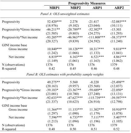
The key prediction of our theoretical framework is that progressivity affects observed inequality differently than it does true inequality, and that the difference between the two inequality effects is increasing with the extent of tax evasion and its responsiveness to tax changes, ceteris paribus. To test this hypothesis, we use a country-level dataset of GINI coefficients calculated separately for gross income, net income, and consumption. We argue that the consumption-based measure of income is closer to true permanent income in comparison to disposable income reported in the household surveys.3
Our empirical analysis reveals that while progressivity reduces observed inequality in reported gross and net income, it has a significantly smaller impact on inequality in consumption. We theorize that the “positive” effect of progressivity on true inequality is possible, especially in the presence of weak legal institutions that can trigger a very large tax evasion response. The evidence provides some support for our
hypothesis as we show that weaker law and order produce a positive effect on inequality in consumption. As expected, we find that progressivity has a larger negative effect on net income inequality than on gross income inequality.
The second essay is an attempt to get a more detailed understanding of the relationship between tax rates and the distribution of income. Numerous researchers have identified the fact that tax payers change their behavior in response to changes in tax rates. While these behavioral changes are at the core of studies that look at efficiency and optimal tax policy4, little is known about their impact on income inequality. The
literature on taxes and income distribution has acknowledged that taxes have a direct effect and an indirect behavioral effect on inequality (Karoly 1994). However, most of the previous studies fail to separate the two effects or identify the driving forces behind the indirect behavioral effect.5
Therefore, the objective of the second essay is to (1) determine the relative size of the direct and indirect effects and (2) determine the relative size of the behavioral
responses that are driving the indirect effect. By relying on estimates of the various behavioral responses, the essay also identifies the true-tax induced-change in inequality. The analysis is done at the micro level using household surveys. The key contribution of this essay is the identification of two main behavioral responses that drive the indirect effect (productivity and compliance). Gramlich, Kasten, and Sammartino (1993) and Altig and Carlstrom (1999)are limited in this respect as they focus primarily on the labor supply response.6 At the same time, the analysis allows us to identify the true changes in the distribution of income.
Another contribution is its implication for the commonly perceived trade-off between efficiency and equity. To see this contribution, it is important to recognize that changes in inequality that arise from changes in evasion are artificial. In other words, observed inequality can increase if a lower tax rate causes rich tax payers to report a relatively greater share of their income. This increase in inequality represents a shift 4 See Saez (2001), Gruber and Saez (2002) and, Kumar (2008) for a description of two branches of the literature that discusses the importance of behavioral changes for efficiency and tax policy design.
5 Alm, Lee, and Wallace (2005) and Poterba (2007) identify the direct and indirect effects while Gramlich, Kasten, and Sammartino (1993) and Altig and Carlstrom (1999) identify some of the behavioral responses that contribute to the indirect effect.
toward the true inequality that existed prior to the tax change. Therefore, to the extent that this “artificial” effect is relatively large, the actual equity cost of the efficiency gained from switching to a flatter tax schedule will be much lower than observed. In this case, it is optimal to adopt a flatter tax schedule not only because it is more efficient but also because negative equity effects are smaller than we think (and possibly positive). Regardless of its size, the evasion (artificial) effect will play an important role in the optimal progressivity debate.
The results are equally interesting if it turns out that the behavioral responses play a minor role in the determination of inequality. Such a result would indicate that the indirect effect is small, which would then imply that the optimal tax schedule may be made more progressive with little efficiency costs. Therefore, knowing if and how taxes affect the distribution of income and consumption is important for policy makers as they attempt to strike an important balance between efficiency and equity.
It is important that we point out at this stage that this dissertation focuses on the personal income tax only. As such, we ignore other aspects of the tax system and their possible feedback effects to the personal income tax. It would be preferable to account for these, but the data requirements cannot be met. In this respect, we follow a long and esteemed literature (Alm and Wallace 2007; Auten and Carroll 1999; Feldstein 1995; Gruber and Saez 2002; Kopczuk 2005).
ESSAY 1: TAX PROGRESSIVITY AND INCOME INEQUALITY
Introduction
The economic literature has long viewed efficiency and equity as two important objectives of economic development. There is also a well established tradeoff between these two objectives; policies that tend to increase efficiency are also likely to increase inequality. This efficiency-equity tradeoff is especially pronounced in income taxation (Mirrlees 1971; Ramsey 1927). It is commonly believed that efficiency is best achieved by the use of simple lump sum taxes that do not distort the choices that people make, whereas vertical equity generally requires progressive tax schedules accompanied by individual specific deductions, allowances, and credits, which are distortionary. As such, taxes that are efficient are thought to reduce equity and vice versa.
But are these two objectives always in conflict? Underlying this tradeoff is the presumption that a higher level of tax progressivity reduces income inequality. It is not difficult to show that a structurally progressive tax (i.e., average tax rate increases with income) results in a more equal distribution of disposable income, assuming no
behavioral responses to tax changes and holding redistribution constant. In reality, however, behavioral responses should not be ignored. For example, increased
progressivity may lead to lower levels of tax compliance among the rich thus increasing their disposable income since they do not pay taxes on the hidden income. An
and is significant, progressivity will have a different effect on observed inequality in reported income than on actual inequality in true income.
Verification of this possible differential effect is becoming increasingly important given the number of countries that have or are considering the implementation of tax reforms with tax structures much flatter than their predecessors. Sabirianova Peter, Buttrick, and Duncan (2010) shows that personal income tax (PIT) structures today have fewer tax brackets, lower top statutory marginal tax rates and reduced complexity than 25 years ago. They also identify what appears to be a shift towards flat rate income taxes. By 2009, 24 countries adopted the flat rate PIT schedule and many more countries are seriously considering this policy. If progressivity and income inequality are negatively related, then there are important implications of such policies for the distribution of income. Given the tax evasion argument, however, it is not clear that shifting to flat taxes – or more generally, to income tax structures with lower levels of progressivity – will necessarily lead to greater levels of income inequality. This is where the distinction between observed and true income distribution and the potential differential effect of progressivity on both becomes extremely important.
period 1981-2005. In this regard, the study is different than most of the previous work, which has been country-specific and relied on micro-simulation exercises or computable general equilibrium models (Gravelle 1992; Martinez-Vazquez 2008). We do
acknowledge that macro analysis has certain limitations as we are not able to examine within country heterogeneity in individual responses or directly estimate the tax evasion effect on income inequality. We also cannot account for the possible offsetting effects of other taxes.7 Nevertheless, macro data provide an exceptional opportunity for cross-country comparisons in testing several important hypotheses.
The key prediction of our theoretical framework is that progressivity affects observed inequality differently than it does true inequality, and that the difference between the two inequality effects is increasing with the extent of tax evasion and its responsiveness to tax changes. To test this hypothesis, we use a country-level dataset of GINI coefficients calculated separately for gross income, net income, and consumption. We argue that the consumption-based measure of income is closer to true permanent income in comparison to disposable income reported in the household surveys. We also develop and estimate comprehensive, time-varying measures of structural progressivity of national income tax systems by using complete national income tax schedules with statutory rates, thresholds, country-specific tax formulas and other information. Our empirical analysis reveals that while progressivity reduces observed inequality in reported gross and net income, it has a significantly smaller impact on inequality in consumption. We theorize that a positive effect of progressivity on true inequality is plausible, especially in the presence of weak legal institutions that can trigger a very large
7 In principle, policy makers could achieve the same level of income inequality by reducing the
tax evasion response. The evidence provides some support for our hypothesis as we show that weaker law and order produce the positive effect on inequality in consumption. As expected, we find that progressivity has a larger negative effect on net income
inequality than on gross income inequality.
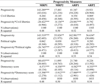
This paper also contributes to the testing of two additional hypotheses. One hypothesis is that an inverted U-shape relationship exists between income inequality and growth; the Kuznets hypothesis. According to Kuznets (1955), this relationship is driven by changes that take place in the allocation of resources as the economy expands. Our results are consistent with this hypothesis. Another hypothesis, derived from the median voter theorem is that democracy and income inequality should be negatively related. While we do not test this hypothesis directly, we do show that progressivity tends to have a larger equalizing effect in societies that are more democratic. We argue that this
reinforcing effect works via larger redistribution which is brought about by the median voter in democratic societies.
The paper proceeds as follows. First, I provide the theoretical framework. This is followed by a description of the data, the empirical model, and the results. The last section concludes.
Theoretical Framework
More progressive taxes are often designed to collect a greater share of income from the rich relative to the poor, thus reducing the inequality of disposable income relative to taxable income. However, as the government increases structural
true income (productivity response) or simply reporting a smaller share of true income (tax evasion/avoidance response) and/or both. While both behavioral responses are likely to reduce observed income inequality, they can have a differential effect on true income inequality. That is, though we expect the productivity response from more progressive taxes to reduce true inequality, the evasion response may increase true disposable income of the rich (since no taxes are paid on the hidden income) and thus increase true
inequality in net income.
The existing estimates of the productivity response based on the labor supply elasticity with respect to tax changes are rather modest (Blundell, Duncan, and Meghir 1998; Eissa and Liebman 1996). However, they may well be understated as they do not account for other forms of productivity adjustment such as response in efforts,
occupational mobility, job reallocation, etc. Another common measure, the elasticity of taxable income, is not a suitable statistic to assess the productivity response as it also blends in the tax evasion response (Chetty 2009). Recently, Gorodnichenko, Martinez-Vazquez, and Sabirianova Peter (2009) (GMP henceforth) propose to use consumption data to measure the productivity response to tax changes; they find a relatively small growth in consumption of wealthier households that faced smaller tax rates after the 2001 Russian flat rate income tax reform. At the same time, they estimate a significant
increase in reported income (5 to 10 times larger than the consumption increase net of windfall gains), attributing the difference to improved tax compliance of households in the upper tax brackets. It has also been argued, in earlier studies, that the
(Feldstein 1995; Slemrod 1994). In other words, the rich tend to be more sensitive to changes in the tax rates because they are better able to hide their income.
If the tax evasion response is indeed large, then the negative effect of higher and more progressive taxes on observed income inequality will significantly overstate (in absolute terms) their effect on true distribution. Below we illustrate these possibilities more formally using both the Kuznets ratio and variance of log income as measures of inequality. We first model the effect of tax progressivity on observed income inequality and then on true income inequality.
We can show these results more formally by starting with a utility maximization problem that allows each person to choose the optimal amount of earned income and the amount of evasion. These utility maximizing quantities should be functions of the tax rate and other parameters and should therefore give us an indication of the effect a change in tax rates will have on the distribution of income. We assume that each individual’s utility function, U(C,y)=C−ψ(y), is concave, increasing in C,
consumption, and decreasing in y, true income (Saez 2001),.8 As specified, the utility function imposes the assumption of strong separability which may be quite
restrictive,(Cowell 1985). However, we follow Chetty (2009)and Saez (2001) in writing the utility function this way; a more general model is derived in the appendix. It is also assumed that each tax payer must make a choice about how much of earned income to evade. This gamble is summarized by the probability of being caught,0≤ρ≤1, and the
penalty structure, , where E is hidden income, t is the tax rate, F is the fine,
and . Therefore, consumption in the two states can be summarized as follows:
) (E F tE+
( )
E1
C
0 / >
F
( )
−t y = 1( )
−t y = 12
C
tE
C1 + 1
F
C2 − 2
where is equal to minus the penalty. Consumption is in state one where the
probability of not being caught is
1
C
(
1−ρ)
, and in state two where the probability ofbeing caught is
2
C
ρ. The individual maximizes expected utility by choosing y, income,
and E, hidden income to solve the following;
( ) (
t y)
tE F( ) ( )
E y Max = 1− + 10 , 0 ≥ ≥ y E ψ ρ
ρ − −
−
EU
subject to
Differentiating with respect to y and E yields
( )
1− /( )
y ≤0= y EU − ∂ ∂ t ψ 3
(
)
ρF/( )
E ≤0)
1− = E
( )
t =ψ/(
ρ)
t=ρ− ∂ ∂ t EU ρ
)
4Assuming we have values that satisfy interior solutions, we can write eq. (3) and (4) as
(
y1− 5
(
E F/1− 6
equal to the marginal benefit of income. The marginal benefit from income is the net of tax expected change in utility that result from the change in y. Similarly, the optimal amount of hidden income is that amount which sets the expected marginal benefit of evasion equal to the expected marginal cost of evasion. These equations can be solved for y and E if a specific utility function is assumed. The expressions for y and E can then be used to construct measures of income inequality that can be used to determine the effect of taxes on the distribution of income.
Inequality in Observed Income
In this subsection, we use two inequality indices that demonstrate the effect of structural progressivity on observed income inequality. Suppose we have two groups of individuals: r=rich and p=poor. Let be observed income inequality in disposable income between rich and poor, measured as the Kuznets ratio, which is the ratio of income received by the rich relative to that received by the poor. We can write the Kuznets measure of observed inequality in disposable income as:
(
)
(
)
( )
or r p o p
r o r o
p o r o
y
Y t t Y
t Y G
y y I
θ
+ −
− =
+ =
1 1
7
where Yo is observed gross earned income reported for tax purposes, y0 is observed earned income net of tax, t is the average tax rate, and G is non-taxable government transfers. For simplicity of exposition, we assume that transfers are exclusively from rich to poor, and that they comprise a fixed portion θ of revenues collected from rich.
also note that observed gross income can be written as the difference between the true income Y* and hidden income E; o r r for rich and for poor.
r Y E
Y = *−
p p o
p Y E
Y = *−
Holding the tax rate facing the poor constant, tr becomes an indicator of structural tax progressivity. Changes in structural progressivity create behavioral responses among
the rich – a likely negative productivity effect 0
* < ∂ ∂ r r t Y
and a positive tax evasion effect
0 > ∂ ∂ r r t E
. These assumptions follow from the earlier discussion. Furthermore, since the
average tax rate facing the poor doesn’t change, we assume no behavioral response for the poor.9
As illustrated below,
r o y t I ∂ ∂
is unambiguously negative under these assumptions.
[
]
(
)
(
)
(
)
21 1 G o p y o r Y r o r Y r r o r Y o r Y r r o r Y G o p y r o y I + + ∂ ∂ − − − − ∂ ∂ + = ∂ ∂ ⎥⎦ ⎤ ⎢ ⎣ ⎡ ⎥ ⎦ ⎤ ⎢ ⎣ ⎡ τ τ τ θ τ τ τ 8
(
)
( )
(
)
22 1 G o p y o r Y o r Y r r o r Y o p y + − − − ∂ ∂ = ⎥⎦ ⎤ ⎢ ⎣ ⎡ θ τ τ
( )
( )
0,2 2 1 * 1 0 0 0 0 < ⎟ ⎠ ⎞ ⎜ ⎝ ⎛ + ⎟ ⎠ ⎞ ⎜ ⎝ ⎛ − ∂ ∂ − − ∂ ∂ − + − = < < < < 4 43 4 42 1 4 4 3 4 4 2 1 43 42 1 3 2 1 t tion effec redistribu effect evasion effect ty productivi effect
direct yop G
o r Y r r E r A r r Y r A o r AY θ τ τ τ τ 9
where
2 ⎟ ⎠ ⎞ ⎜
⎝
⎛ +
=
G o
p y
o p y
A . The first term in eq. (9) shows the direct effect of tax
progressivity on income inequality in the absence of behavioral responses and subsequent redistribution from rich to poor. The negative direct effect arises simply from the fact that a progressive tax structure imposes a relatively higher tax burden on the rich.
Equation (9) hints that the response of true and observed inequality to tax changes is likely to be different. Because the rich have greater access to the various means of hiding their income, they report a relatively smaller share of their income as structural progressivity increases, which give the false impression that the distribution of income is becoming more equal. As shown below, however, the distribution of true income may not improve.
The last term in eq. (9) shows the negative redistribution effect. If the
government succeeds in redistributing the collected revenues in a pro-poor or neutral manner, then the higher taxes on the rich are likely to reduce observed income inequality,
ceteris paribus. On the other hand, if redistribution is pro-rich, then the effect of structural progressivity on observed income inequality becomes ambiguous.
Thus, the negative direct effect of higher tax progressivity on observed income inequality is reinforced by the negative productivity response, the positive tax evasion response, and pro-poor redistribution. Consequently, we formulate two hypotheses that can be tested with macro data:
Hypothesis 1The statistical relationship between tax progressivity and income
Hypothesis 2Factors that are positively associated with pro-poor redistribution such as
democracy and civil liberties (Meltzer and Richard 1983) are likely to reinforce the
negative effect of structural tax progressivity on observed income inequality.
Similar to the Kuznets ratio explored above, the effect of taxes on the distribution of income can be obtained by differentiating the variance of log net income index with respect to taxes. We write the variance of log net income as10.
(
)
(
)
∑ − = ⎟ ⎠ ⎞ ⎜ ⎝ ⎛ = = n i i o μ y n o y VLI 1 2 2 ~ log log 1 log var 10 where = ∑(
= n i o i y n μ 1log 1 ~
log
)
is the mean of log income. Totally differentiating eq. (10) withrespect to ti yields the following.11
(
)
(
( )
)
(
)
(
i i)
ii i Ei i yi i n i i o
i μ y Y E Y E d
y n VLI d τ τ τ ε ε ⎥ ⎥ ⎦ ⎤ ⎢ ⎢ ⎣ ⎡ − − ⎟⎟ ⎠ ⎞ ⎜⎜ ⎝ ⎛ − − ∑ − = − = * * 1 1 1 ~ log log 2 11 which we rewrite as
( )
(
)
(
i)
ii i Ei i yi n
i Ai d
n
VLI
d π τ
τ τ ε π ε ⎥ ⎥ ⎦ ⎤ ⎢ ⎢ ⎣ ⎡ − − ⎟⎟ ⎠ ⎞ ⎜⎜ ⎝ ⎛ − − ∑ =
= 2 1 1
1
12
where
(
( )
)
(( )) 1 1 1 ~ log log − − − − = i i o ii y μ
A π τ , * i i i Y E =
π , and
j t t j j ∂ ∂ =
ε is the elasticity of j (evasion or
income) with respect to taxes.
It is clear from eq. (12) that the net effect of taxes on inequality depends on the sum of its effect on the various parts of the income distribution. While the sign of the
10 Since y and E are derived from the maximization problem they are functions of the tax rate, and the other parameters specified in that problem. Note also, that we ignore transfers for this exercise. They can be easily included; see appendix A.
term in square brackets is likely to be negative for everyone (as discussed in more detail later), the sign of the first term varies along the income distribution. It is negative for those earning less than mean income and positive for those earning more than mean income. Therefore, reducing the tax rate on individuals above mean income should increase income inequality, while reducing taxes on those below mean income should reduce inequality. The net effect will depend on which of these two effects dominates.12 This finding is consistent with the previous literature. In particular, it is commonly known that the impact of any tax reform on the distribution of income depends on the existing income distribution (Fuest, Peichl, and Schaefer 2008; Poterba 2007).
Equation (12) also shows that taxes affect inequality through direct and indirect channels. The direct effect is captured by the term
(
1−πi)
while the tax-induced indirecteffects are captured by
(
)
⎟⎟ ⎠ ⎞ ⎜⎜ ⎝ ⎛ − −i i Ei i
yi τ
τ ε
π
ε 1 , which includes both the productivity effect,
yi
ε and the evasion effect, πiεE. Now, to see the distributional impact of a tax reform,
let us assume that dti=0 foreveryone below mean income, dti<0 for those above mean income, εyi <0, andεE >0.
13 Under these assumptions, all three channels contribute to
an unambiguous increase in observed net income inequality. This result is due to the fact that both the evasion and productivity responses lead to a relative increase in reported gross income for the rich, which in turn leads to an increase in observed net income inequality. The direct effect is also straightforward; the lower rates on the rich reduce
12 Obviously, if a tax reform involves reducing top rates only, the change in inequality will be positive. This assumes that the top rate applies only to individuals whose income is above the mean.
13We make these assumptions to simplify the discussion. Note that A
i is positive for these individuals.
their tax burden relative to the tax burden facing the poor thus resulting in an increase in net income inequality.
Inequality in True Income
We now turn our attention to true income inequality. Using the above notations, we define true income inequality as the ratio of actual disposable income received by
the rich relative to that received by the poor:
*
y
I
(
)
(
)
( )
or r p p o p r r o r p r
y Y E Y
E Y G y y I τ θ τ τ + + − + − = + = 1 1 * * * 13 We again assume that redistribution is pro-poor (0<θ<1). Given that true income
is the sum of reported income and hidden income, i.e., , we can obtain the following partial effect of structural progressivity on true income inequality, holding tax rates of the poor and redistribution policy
r o r
r Y E
Y*= +
p
t θ constant.
(
)
G y Y t Y t G y y t E Y t t Y t I p o r r o r r p r r r o r r r o r r y + ⎥ ⎦ ⎤ ⎢ ⎣ ⎡ + ∂ ∂ + − ⎥ ⎦ ⎤ ⎢ ⎣ ⎡ ∂ ∂ + − − ∂ ∂ = ∂ ∂ * * ** 1 θ
14
(
) (
)(
)
(
)
G y I t E I E Y t I t t Y t I p y r r r y r r r y r r o r r y + ⎥ ⎦ ⎤ ⎢ ⎣ ⎡ + ∂ ∂ + + − − − − ∂ ∂ = ∂ ∂ * * * * ** 1 θ 1 θ τ 1 θ
15
(
)
[
(
)
(
)
]
0 1 1 1 * * * * * * > < + + − + + + ∂ ∂ = ∂ ∂ G y Y E I t Y t I p t r Et r y r r r y ε ε θ 16 whereεEt >0 and ε*t >0 is the elasticity of evasion and true income with respect to taxEquation (16) demonstrates that the effect of tax progressivity on true income inequality is ambiguous. Higher taxes on the rich could increase actual income inequality if the share of hidden income among the rich is large while the elasticity of true
income/productivity is small relative to the elasticity of hidden income. For example, GMP find a large positive tax compliance response but small productivity/consumption response of affluent households to Russia’s 2001 flat rate personal income tax reform. Thus, in countries like Russia, inequality might possibly decline from lowering upper tax rates.
While we do not observe true income in a typical household survey, we agree withGMP that expenditures or consumption are more difficult to hide, and are therefore much closer to true permanent income than is reported income. The testable implication is that in the presence of a positive tax evasion response, an increase in structural
progressivity should bring a more sizeable reduction in observed income inequality than in consumption inequality. A positive effect on consumption inequality is also possible.
Another important implication of eq. (16) is that the difference between the effect of tax changes on consumption inequality and their effect on observed income inequality is expected to increase with the extent of tax evasion. Assuming that the weakness of legal institutions is positively correlated with the share of hidden income, we may anticipate that a positive effect of structural progressivity on consumption inequality is more likely to be found in countries with weaker legal institutions.
Hypothesis 3The effect of structural progressivity on inequality in consumption is likely
to be smaller than the effect of structural progressivity on inequality in observed net
income. A positive effect on consumption inequality is possible.
Hypothesis 4The positive effect of structural progressivity on consumption inequality is
more likely to be found in countries with weaker legal institutions.
Similar conclusions are reached using the variance of log income to assess the impact of changes in progressivity on income inequality. To see this, first write true net income as
(
i)
i i ii t Y tE
y*= 1− *+
17
Totally differentiate eq. (10) with * replacing to get
i
y o
i
y
( )
(
( )
) (
)
Ei(
i i)
ii i i i Ei i yi i n
i i i t y E dt
E t t E y y μ y n VLI d ⎥ ⎦ ⎤ ⎢ ⎣ ⎡ − − + ⎟⎟ ⎠ ⎞ ⎜⎜ ⎝ ⎛ − − ∑ − = − = * * 1 1 *
* log~ 1
log
2 ε ε ε
18 While the sign of the first term,
(
log( )
yi logμ~)
* −
dt
, varies along the income distribution as in the previous section, the sign of the last term is now ambiguous. Therefore, it is possible for a reduction in the tax rate, for example, to reduce inequality. This possibility is greatest when evasion is widespread and is very responsive (positively) to the tax rate. To see this, we order individuals according to income from lowest to highest. Let n1 individuals have income lower than mean income and N-n1 individuals have income above mean income. Now, suppose that i is negative for all i∈
[
n1+1,N]
and zero for alli∈
[
1,n1]
. This implies that eq. (18) can be rewritten as( )
(
( )
)
[
(
)
]
i Ei(
i)
ii i yi N
n
i i i i i t dt
t t t μ y n VLI d ⎥ ⎦ ⎤ ⎢ ⎣ ⎡ − − + ⎟⎟ ⎠ ⎞ ⎜⎜ ⎝ ⎛ − ∑ − − + + = −
= 2 log log~ 1 π ε 1 πε 1 π
1
1 *
1
which is negative if the evasion effect is positive and larger than the other two terms in the square bracket. That is, reducing the tax rate reduces income inequality. The
implication of this result is that the shift to flatter personal income tax schedules that has taken place over the last two decades may have led to an improvement in the distribution of actual net income in countries where the “right” conditions exist. As such, we can derive similar hypotheses to those derived using the Kuznet Ratio.
The theoretical discussion above tells a compelling story about the possible distributional impact of tax reforms and how such effects should be evaluated. In particular, it points to the need to distinguish between direct and indirect effects by acknowledging the role played by behavioral responses, and between actual and observed net income inequality by acknowledging the role played by evasion. Ignoring these distinctions can lead to seriously misguided policy prescriptions. For example, whereas a reduction in tax rates can be expected to increase observed net income inequality, it can also reduce actual net income inequality. Similarly, the evasion response is shown to affect observed net income inequality differently than it does actual net income
inequality; the evasion effect leads to increased observed inequality but may lower true inequality, ceteris paribus. An empirical analysis is therefore required to identify the sign and size of the various channels discussed above.
Measuring Inequality and Structural Progressivity
Income Inequality Measure
v.2b), the International Labor Office LABORSTA, and European Commission
EUROSTAT. Altogether these sources provide us with 3512 GINI estimates from 1981 to 2005. For the purpose of our analysis, we selected all GINI coefficients that are based on one of the three income definitions: gross income, disposable (net) income, and expenditures or consumption. The selected GINIs were grouped into 3 categories of area coverage (national, urban or national with exclusions, and other), 4 categories of income adjustment (equivalence scale, per capita adjustment, no adjustment, and unknown), and 4 categories of data quality rating.14 We then averaged multiple GINI measures by country, year, income base, area coverage, income adjustment, and quality rating. Finally, for a given country, year, and income base, we selected one average measure using the following set of preferences: national estimates are preferred to urban, rural and other area coverage estimates, equivalence scales or per capita adjustment are chosen over no or unknown adjustment, and higher quality GINIs are preferred to those with lower quality.
This selection process left us with 1683 GINI estimates for 143 countries from 1981 to 2005.15 The majority of the estimates meet the best practices as set out by the WIDER. Appendix Table B 1 shows that 93 percent of the GINI estimates have national coverage, 75 percent have been adjusted for the household size, and 71 percent have a good quality rating, 1 or 2. Also, the distribution across income base is suited for the type of analysis that we carry out in the paper. More specifically, of the total sample of
14 The data quality rating is designed by the WIDER. It ranges from 1 to 4, where 1 denotes observations with a sufficient quality of the income concept and the survey. As to other data sources, we assigned 1 to Eurostat data and 2 to ILO estimates.
GINI estimates, 20 percent are based on consumption, 34 percent on gross income, and 46 percent on net income. To control for differences in GINI measurement, our estimates include dummy variables for income base, area coverage, and income adjustment
categories. While we recognize that the use of dummy variables does not eliminate all of the biases resulting from comparability issues (Atkinson and Brandolini 2001), we are constrained by existing inequality estimates. This is especially restricting in cross-country panel studies due to variations in the quality of primary data sources, differences in definition of variables and other procedures followed by individual countries.
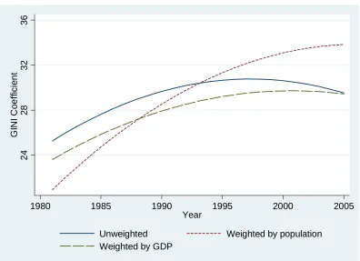
In an effort to identify the trend in income inequality over time, we regress the GINI coefficients on a quadratic time trend, controlling for income base, area coverage, income adjustment, and country classification.16 The coefficients on the time terms are then used to plot the average GINI trend in Figure 1. The results indicate that income inequality increased throughout the 1980s and 1990s before declining during the 2000– 2005 period. Figure 1 also reports the time trend weighted by a country’s GDP in constant U.S. dollars and population.17 While the GDP–weighted trend follows that of the unweighted, the population–weighted trend shows income inequality increasing throughout the sample period, which is consistent with rising inequality in China, India, and other developing countries with large populations.
16 A similar, though not identical, procedure is used by Easterly (2007) to address the consistency problem inherent in the GINI data. Country categories are defined using the World Bank country classification based on historical (time-varying) income thresholds. For example, the income thresholds used for the 2005 classification are as follows: low income, $875 or less, lower middle income, $876-$3465, upper middle income, $3466-$10725, and high income, $10725 or more.
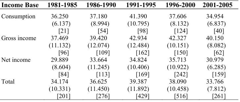
Table 1 provides additional summary statistics on the GINI coefficient by income definition across time. However, one has to be careful in interpreting these numbers because of comparability issues. In particular, the income–based and expenditure–based measures cannot be compared without a regression framework because the latter
Figure 1. Global Trend in Income Inequality, 1981-2005
24
28
32
36
G
INI
Co
ef
fi
c
ie
n
t
1980 1985 1990 1995 2000 2005
Year
Unweighted Weighted by population
Table 1. Average GINI by Income Base and Period
Income Base 1981-1985 1986-1990 1991-1995 1996-2000 2001-2005
Consumption 36.250 37.180 41.390 37.606 34.954
(6.137) (8.994) (10.795) (8.132) (6.837)
[21] [54] [98] [124] [40]
Gross income 37.469 39.420 42.934 42.327 40.150
(11.132) (12.074) (12.484) (10.151) (8.082)
[96] [109] [162] [150] [62]
Net income 29.889 33.664 34.824 35.713 30.979
(8.604) (11.245) (10.406) (10.922) (6.285)
[84] [113] [169] [242] [159]
Total 34.174 36.625 39.387 38.090 33.766
(10.331) (11.450) (11.892) (10.458) (7.812)
[201] [276] [429] [516] [261]
Notes: Number of GINI observations is 1683; number of country-year observations is 1229. Standard deviation is in parentheses and number of GINI observations is in brackets.
Tax Progressivity Measures
In contrast to income inequality, the measures of tax progressivity are not readily available for cross-country comparison. The existing measures implemented in the literature fall into one of three groups: (1) the top statutory PIT rate, (2) effective
inequality-based measures of progressivity, and (3) structural progressivity measures. In their original form, none of these measures are perfectly suitable for our analysis.
that will be introduced below. For that reason, we do not discard this variable and will employ it in some specifications.
The effective progressivity is based on some indicator of income inequality. In its simplest form, effective progressivity is the ratio of after-tax GINI to before-tax GINI and “measures the extent to which a given tax structure results in a shift in the distribution of income toward equality” (Musgrave and Thin 1948). More sophisticated measures have been proposed by Kakwani, (1977) Suits (1977), and others. The inequality-based measures generally require information on pre-tax and post-tax inequality and the distribution of the tax burden. Information on these variables is either not available or not comparable across countries. The more serious problem, though, is the issue of simultaneity in determination of income inequality and inequality-based progressivity, which inhibits the identification of the direct effect of tax progressivity on inequality.
Ideally we need a single, comprehensive measure of PIT progressivity, which is comparable across countries, available for a large representative sample of countries, and vary over time. We propose the following procedure to derive such a measure.
The first step in calculating structural progressivity is to obtain average and marginal tax rates at different points of the income distribution. Instead of actual income distribution, we use a country’s GDP per capita and its multiples as a comparable income base. The GDP figures are rescaled to get 100 units of pre-tax income for each country and year, ranging from 4 percent to 400 percent of a country’s GDP per capita. We then apply the tax schedule information to these units of income to obtain tax liability and average and marginal tax rates. The data on national tax schedules is collected for 189 countries from 1981 to 2005 and described in detail in Sabirianova Peter, Buttrick, and Duncan (2010). Here we just note that our average and marginal tax rates take into account standard deductions, basic personal allowances, tax credits, local taxes, major national surtaxes, multiple schedules, non-standard tax formulas, and other provisions in addition to statutory rates and thresholds.
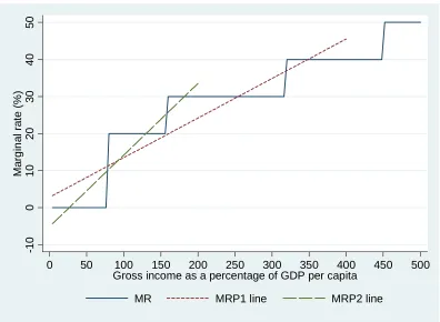
The progressivity measures are obtained by regressing marginal (or average) rates on gross income using 100 data points that are formed around a country’s GDP per capita in a given year. The slope coefficient on the income variable measures the percentage point change in the tax rate resulting from a one percentage point change in pre-tax income18 and is our measure of structural progressivity. The PIT structure is interpreted
as progressive, proportional or regressive if the slope coefficient is positive, zero or negative, respectively. This procedure gives us marginal rate progression (MRP1) and
average rate progression (ARP1) for each country and year in our dataset. Figure 2 illustrates how the MRP1 is obtained for a hypothetical case with no allowances and other provisions.
It should be noted that structural progressivity can deviate significantly from the nominal progressivity of the legal tax scale. This is especially pertinent to low income countries, where taxable income of the majority of population is often below the first tax threshold. Based on our procedure, countries for which a significant proportion of the population does not pay taxes will have progressivity measures of zero or close to zero. This makes sense, since the tax structure is effectively proportional when no one is paying taxes, even if the statutory rate schedule is highly graduated.
To obtain a single, comprehensive measure we had to impose a linearity
restriction on the relationship between rates and income levels. Given that the nominal tax schedule has a top statutory marginal rate, both the average and marginal rate progression measures, as defined by Musgrave and Thin , decline as one move up the income distribution. In other words, the tax schedule is less progressive at the top of the income scale. In an effort to capture this nonlinearity, we also calculated MRP2 and ARP2 for the bottom portion of the income scale up to 200 percent of a country’s GDP per capita. Figure 2 illustrates MRP2 for a hypothetical case
Figure 2. Marginal Rate Progression: Illustrative Example
-1
0
0
10
20
30
40
50
Ma
rg
in
a
l ra
te
(%
)
0 50 100 150 200 250 300 350 400 450 500
Gross income as a percentage of GDP per capita
MR MRP1 line MRP2 line
Notes: Figure 2 depicts a hypothetical schedule of marginal rates (MR), with top statutory PIT rate 50 percent and no deductions and tax credits. Marginal rate progression (MRP) is the
estimated slope coefficient from regressing marginal rates on gross income (as percent of GDP per capita). MRP1 is calculated for gross income from 4 percent to 400 percent of y, MRP2 is calculated for gross income from 4 percent to 200 percent of y, where y is a country’s GDP per capita.
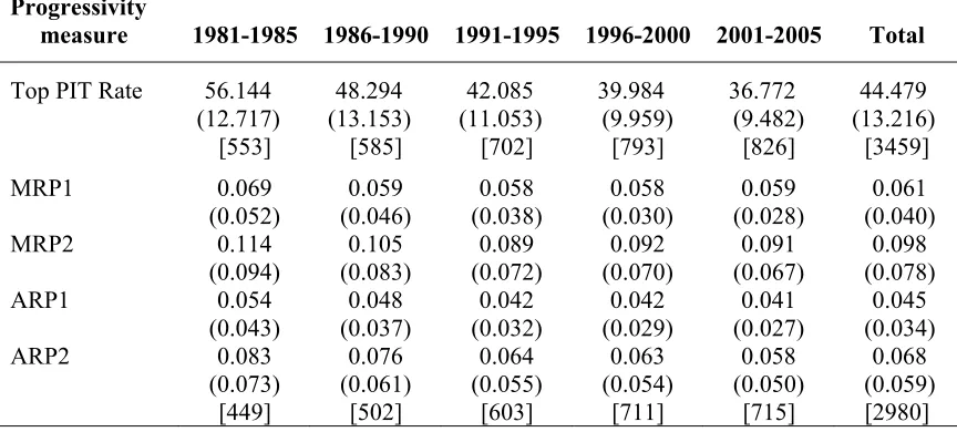
Table 2 reports summary statistics on four progressivity measures across time. To infer the global trend, mean values are weighted by a country’s share in world GDP and world population. The pattern that stands out is that all of the measures declined
measures. Table 2 also reports summary statistics on the top statutory PIT rate. The top marginal tax rate has declined steadily from a high of 56 percent in the 1981–1985 period to a low of 37 percent in the 2001–2005 period. Since these global trends follow closely those reported in Sabirianova Peter, Buttrick, and Duncan (2010), we refer the reader to that paper for a more detailed description of the changes that have taken place over the last 25 years.
Table 2. Structural PIT Progressivity by Period
Progressivity
measure 1981-1985 1986-1990 1991-1995 1996-2000 2001-2005 Total
Top PIT Rate 56.144 48.294 42.085 39.984 36.772 44.479
(12.717) (13.153) (11.053) (9.959) (9.482) (13.216) [553] [585] [702] [793] [826] [3459]
MRP1 0.069 0.059 0.058 0.058 0.059 0.061
(0.052) (0.046) (0.038) (0.030) (0.028) (0.040)
MRP2 0.114 0.105 0.089 0.092 0.091 0.098
(0.094) (0.083) (0.072) (0.070) (0.067) (0.078)
ARP1 0.054 0.048 0.042 0.042 0.041 0.045
(0.043) (0.037) (0.032) (0.029) (0.027) (0.034)
ARP2 0.083 0.076 0.064 0.063 0.058 0.068
(0.073) (0.061) (0.055) (0.054) (0.050) (0.059) [449] [502] [603] [711] [715] [2980] Notes: Standard deviation is in parentheses and number of country-year observations is in brackets.
Empirical Methodology
The OLS Model for Observed Income Inequality
Following the theoretical model discussed above, we write observed income inequality as a function of structural progressivity and other control variables:
it it it it t
it P Z W
I =ξ +β +δ +φ +ε 20
where Iit is observed inequality measured by income-based GINI coefficients (either net or gross income) in country i and year t, ξt captures year effects, Pit is the relevant
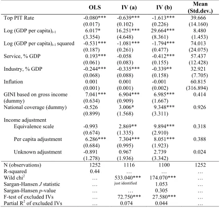
measure of PIT progressivity, Zit is a vector of control variables, and Wit is a vector of auxiliary variables that are included to control for consistency of the GINI coefficients (a dummy for national area coverage, a set of dummies for the type of income adjustment, and a dummy to indicate the type of income base (gross or net income), and εitis the error term. The Z vector includes the one-year lagged log of GDP per capita in quadratic form, the rate of inflation, the share of services in GDP, and the share of industry in GDP (see Appendix Table B 2 for variable definitions). The quadratic form of GDP per capita is used to account for the existence of the Kuznets Curve which postulates that there is a non-linear (inverted U) relationship between income inequality and per capita GDP. If it exists, we expect a positive coefficient on the linear term and a negative coefficient on the quadratic term. The coefficient of interest, β, captures the effect of progressivity on inequality in observed income, and is expected to be negative.
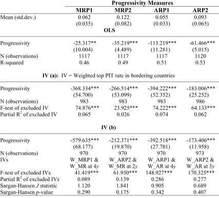
GINI by 0.08 points, ceteris paribus.19 Inequality in gross income is predictably higher than inequality in net income. The sign of the coefficients on both GDP terms is consistent with the Kuznets hypothesis. Table 4 includes the same set of covariates as in Table 3, except for the top statutory PIT rate, which is replaced with one of the
measures of structural progressivity. All of the progressivity measures have a statistically significant negative effect on income inequality. However, the magnitude of the
marginal effects is small. A 100 percent increase in any progressivity measure reduces the GINI coefficient by less than 20 percent at the mean. For example, a twofold increase in the MRP1 slope from 0.062 (mean) to 0.124 is estimated to reduce the GINI
coefficient by 1.57 (=25.317*0.062); not such a large effect given that the sample mean of GINI coefficients for net and gross income is 37.
Table 3. Base Specification for Inequality in Observed Income
OLS IV (a) IV (b) (Std.dev.) Mean
Top PIT Rate -0.080*** -0.639*** -1.613*** 39.666
(0.017) (0.102) (0.226) (14.160)
Log (GDP per capita)t-1 6.017* 16.251*** 29.664*** 8.480
(3.354) (4.648) (8.361) (1.453)
Log (GDP per capita)t-1 squared -0.531*** -1.081*** -1.794*** 74.013
(0.187) (0.261) (0.477) (24.075)
Service, % GDP 0.193*** -0.058 -0.412*** 57.437
(0.061) (0.083) (0.155) (12.428)
Industry, % GDP -0.244*** -0.335*** -0.339** 32.921
(0.068) (0.088) (0.158) (7.705)
Inflation 0.001 0.001 -0.001 60.815
(0.001) (0.001) (0.002) (316.894)
GINI based on gross income 7.041*** 6.904*** 6.985*** 0.414
(dummy) (0.634) (0.909) (1.667)
National coverage (dummy) -0.526 3.006* 9.348*** 0.926
(0.899) (1.568) (3.311)
Income adjustment
Equivalence scale -0.993 2.869** 9.894*** 0.318
(0.674) (1.335) (2.910)
Per capita adjustment 6.286*** 7.304*** 8.051*** 0.388
(0.684) (0.995) (1.923)
Unknown adjustment -0.891 0.967 2.739 0.024
(1.278) (1.936) (3.342)
N (observations) 1252 1116 1100 1252
R-squared 0.44 … … …
Wild chi2 … 533.040*** 174.070*** …
Sargan-Hansen J statistic … just identified 1.053 …
Sargan-Hansen p-value … … 0.305 …
F-test of excluded IVs … 72.750*** 27.580*** …
Partial R2 of excluded IVs … 0.074 0.044 …
Notes: Robust standard errors are in parentheses; * significant at 10%; ** significant at 5%; ***
significant at 1%. The dependent variable is GINI in gross or net income. Year dummies are included in all three models but not shown here. Instrument in (a) is the distance-population weighted top PIT rate in bordering countries. Instruments in (b) are distance-population weighted MRP1 and marginal rate at income 4⋅y in neighboring countries, where y is a country’s GDP per capita. The omitted category for income adjustment is “no adjustment”
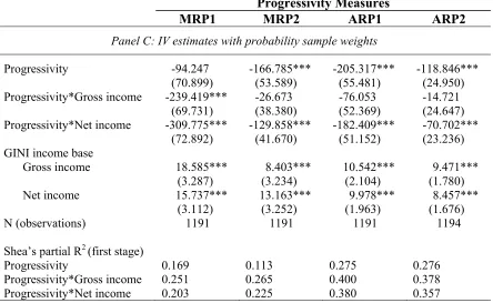
Table 4. Structural Progressivity and Inequality in Observed Income
Progressivity Measures
MRP1 MRP2 ARP1 ARP2
Mean (std.dev.) 0.062 0.122 0.055 0.093
(0.035) (0.082) (0.033) (0.065)
OLS
Progressivity -25.317** -35.219*** -113.219*** -61.466***
(10.004) (4.489) (11.281) (5.015)
N (observations) 1117 1117 1117 1120
R-squared 0.46 0.49 0.51 0.53
IV (a): IV = Weighted top PIT rate in bordering countries
Progressivity -368.334*** -266.514*** -394.222*** -183.006***
(54.700) (53.099) (52.352) (25.252)
N (observations) 983 983 983 986
F-test of excluded IV 74.876*** 23.925*** 74.222*** 64.133***
Partial R2 of excluded IV 0.065 0.026 0.074 0.062
IV (b)
Progressivity -579.635*** -212.371*** -392.518*** -173.406***
(68.177) (19.870) (27.781) (11.958)
N (observations) 970 970 970 973
IVs W_MRP1 &
W_MR at 4y
W_ARP2 & W_MR at 2y
W_ARP1 & W_AR at 4y
W_ARP2 & W_AR at 3y
F-test of excluded IVs 41.419*** 61.930*** 148.927*** 170.325***
Partial R2 of excluded IVs 0.089 0.139 0.286 0.277
Sargan-Hansen J statistic 1.120 1.841 0.905 0.689
Sargan-Hansen p-value 0.290 0.175 0.342 0.407
The IV Model for Observed Income Inequality
Despite the promising start, there are several reasons to believe that the OLS results reported in the previous section might be biased and inconsistent. For example, the ideal estimating procedure would be to use country fixed effects to account for heterogeneity among countries. However, the use of fixed effects is problematic given the limited within variation in the dependent variable for some countries. The GINI data are mostly sparse for a number of the countries in our sample.20 To the extent that constant country characteristics are correlated with the error term, omitted fixed effects create an endogeneity bias.
Another form of endogeneity bias stems from the fact that structural progressivity by itself is an estimated parameter with associated standard errors. This can lead to an attenuation bias in the estimated effects, assuming that standard errors follow the properties of the classical error-in-variables problem.
Finally, an endogeneity bias may arise from reverse causality. The political economy literature has long established a reverse relationship between income inequality and taxes (Meltzer and Richard 1981; Persson and Tabellini 2002). Also, much of the empirical work that examines the effect of income inequality on economic growth argues that inequality affects growth through its effect on taxes and redistribution,(Barro 2000; Milanovic 2000; Perotti 1992; Persson and Tabellini 1994). The general argument, based on the median voter hypothesis, is that as the ratio of median income to mean income falls (i.e., inequality increases), the median voter will vote for higher taxes and greater