www.hydrol-earth-syst-sci.net/12/1007/2008/ © Author(s) 2008. This work is distributed under the Creative Commons Attribution 3.0 License.
Earth System
Sciences
An integrated model for the assessment of global water resources –
Part 1: Model description and input meteorological forcing
N. Hanasaki1, S. Kanae2, T. Oki2, K. Masuda3, K. Motoya4, N. Shirakawa5, Y. Shen6, and K. Tanaka7 1National Institute for Environmental Studies, Japan
2Institute of Industrial Science, University of Tokyo, Japan 3Frontier Research Center for Global Change, Japan
4Faculty of Education and Human Studies, Akita University, Japan
5Graduate School of Systems and Information Engineering, University of Tsukuba, Japan 6Center for Agricultural Resources Research, The Chinese Academy of Sciences, China 7Disaster Prevention Research Institute, Kyoto University, Japan
Received: 17 September 2007 – Published in Hydrol. Earth Syst. Sci. Discuss.: 2 October 2007 Revised: 7 May 2008 – Accepted: 30 June 2008 – Published: 29 July 2008
Abstract. To assess global water availability and use at a
subannual timescale, an integrated global water resources model was developed consisting of six modules: land sur-face hydrology, river routing, crop growth, reservoir opera-tion, environmental flow requirement estimaopera-tion, and anthro-pogenic water withdrawal. The model simulates both natural and anthropogenic water flow globally (excluding Antarc-tica) on a daily basis at a spatial resolution of 1◦×1◦ (lon-gitude and latitude). This first part of the two-feature re-port describes the six modules and the input meteorologi-cal forcing. The input meteorologimeteorologi-cal forcing was provided by the second Global Soil Wetness Project (GSWP2), an in-ternational land surface modeling project. Several reported shortcomings of the forcing component were improved. The land surface hydrology module was developed based on a bucket type model that simulates energy and water balance on land surfaces. The crop growth module is a relatively simple model based on concepts of heat unit theory, poten-tial biomass, and a harvest index. In the reservoir operation module, 452 major reservoirs with>1 km3each of storage capacity store and release water according to their own rules of operation. Operating rules were determined for each reser-voir by an algorithm that used currently available global data such as reservoir storage capacity, intended purposes, simu-lated inflow, and water demand in the lower reaches. The environmental flow requirement module was newly devel-oped based on case studies from around the world. Simulated
Correspondence to: N. Hanasaki ([email protected])
runoff was compared and validated with observation-based global runoff data sets and observed streamflow records at 32 major river gauging stations around the world. Mean annual runoff agreed well with earlier studies at global and conti-nental scales, and in individual basins, the mean bias was less than±20% in 14 of the 32 river basins and less than±50% in 24 basins. The error in the peak was less than±1 mo in 19 of the 27 basins and less than±2 mo in 25 basins. The per-formance was similar to the best available precedent studies with closure of energy and water. The input meteorological forcing component and the integrated model provide a frame-work with which to assess global water resources, with the potential application to investigate the subannual variability in water resources.
1 Introduction
annual water availability or the ratio of withdrawal to avail-ability on an annual basis. However, extreme seasonality in both water availability and water use occurs in some parts of the world. For example, in the Asian monsoon region, con-ditions change dramatically between the rainy and dry sea-sons. Moreover, global warming is projected to alter future temperature and precipitation patterns and consequently af-fect both the amount and timing of water availability and use (Kundzewicz et al., 2007). Therefore, subannual variability must be taken into account.
A model suitable for such assessments requires the follow-ing three functions. First, it must simulate both renewable freshwater resources and water use at a subannual timescale. Second, it must deal with major interactions between the nat-ural hydrological cycle and anthropogenic activities. For ex-ample, withdrawal from the upper stream affects availability in the lower stream, and reservoir operation may contribute to increased water availability in the lower stream. Third, it must explain key mechanisms regarding the effects of global warming on water availability and water use for future pro-jections.
Several integrated global water resources models that can simulate not only the natural water cycle, but also an-thropogenic water flow, have been published. Alcamo et al. (2003a, 2003b) developed a global water assessment model called “WaterGAP 2” which consists of a global wa-ter use model and a global hydrology model, and assessed the current and future water resources globally. Haddeland et al. (2006) developed and implemented a reservoir model and an irrigation model in the Variable Infiltration Capac-ity (VIC) land surface model (Liang et al., 1994) and stud-ied the effects of reservoirs and irrigation water withdrawal on continental surface water fluxes for part of North Amer-ica and for Asia. Jachner et al. (2007) enhanced the LPJmL (Lund-Potsdam-Jena managed land) dynamic global vegeta-tion model (Bondeau et al., 2007) with a river routing model, including lakes and reservoirs, and withdrawals for house-holds and industry, and assessed how much water is con-sumed by global irrigated and rain-fed agriculture and by natural ecosystems. Several other global hydrological mod-els have been developed, but most have focused on the natu-ral hydrological cycle, with less emphasis on anthropogenic aspects.
In contrast to earlier works, we set three basic policies. First, our primary purpose was to assess global water avail-ability and use at a subannual timescale. No previous stud-ies set this as their primary purpose. Second, both water and energy balances on the land surface are closed in our model. This is not only the most fundamental considera-tion of hydrology, but is also one of the key requirements for the interdisciplinary coupling of submodules (e.g., hydro-logical models and crop growth models). Recently, several advanced earth system modeling efforts have been reported such as coupling a land surface model (LSM) with a crop model (Gervois et al., 2004; Mo et al., 2005) and coupling a
global climate model (GCM) with a crop model (Osborne et al., 2007). In these systems, soil moisture, evaporation, and other variables are shared by more than one submodel; there-fore, to maintain consistency among submodels, energy and water balances should be conserved. In particular, the closure of the energy balance is a fundamental requirement of GCM and LSM approaches. Third, as much as possible, we tried to avoid model calibration involving the fit of simulated results to available observation records. Only two hydrological pa-rameters were tuned by climatic zones, not individual basins (Sect. 3.1). It is well established that hydrological models do not reproduce observed hydrographs very well without model calibration (or model parameter tuning). However, in global-scale hydrological modeling, model calibration is a difficult issue. There are a few reasons for this. First, it is virtually impossible to calibrate the model worldwide be-cause of the limited availability of observations, especially in developing countries. Second, both models and input me-teorological forcing and validation data contain considerable uncertainty (Oki et al., 1999), and it is not always easy to at-tribute errors in simulations to improper settings of model pa-rameters. Moreover, we intended to apply the model to future projection under climate change. Thus, the transparency and physical validity of the model are quite important because the simulated results are highly model dependent. Therefore, we extensively examined the simulated results of the model using model inherent parameters; even this sometimes pro-duces large errors.
We developed an integrated global water resources model consisting of six modules: land surface hydrology, river rout-ing, crop growth, reservoir operation, environmental flow re-quirements, and anthropogenic water withdrawal. The model simulates both natural and anthropogenic water flow globally (excluding Antarctica) at a spatial resolution of 1◦×1◦ (lon-gitude and latitude) at a daily time interval.
there are other issues to consider, we started with these six modules that we judged to be most essential for our goal.
The modeling of anthropogenic activities is in its very ini-tial stage in terms of global hydrological modeling. We do not expect that our model can reproduce individual events in the real world. What we introduced into our model was the minimum basic anthropogenic activities in current global hy-drological models; such basic anthropogenic activities are in-dispensable in analyzing the seasonality of water availability and water use. Here, we assume that humans act rationally. We do not expect that our model can reproduce the daily op-eration of individual reservoirs or daily irrigation practices at individual farms in the real world. However, reservoir op-erators seldom release water in floods, and farmers seldom sow in periods that are unsuitable for cropping. Historical reservoir operations were fairly reproduced using a simplis-tic model that assumes rational actions by humans (Hanasaki et al., 2006).
There are two potential beneficiaries of this model: the climate change impact assessment community and the earth system modeling community. A number of global water re-sources models contributed climate change impact projec-tions to the fourth assessment report (AR4) of the Intergov-ernmental Panel on Climate Change (IPCC; Kundzewicz et al., 2007). The global water resources assessments of AR4 were on an annual basis and projected the effects of annual to decadal changes in precipitation and temperature on water resources. However, the effects of subannual change (e.g., decrease in snowfall, earlier snowmelt, increase in the inten-sity and frequency of heavy precipitation, and change in the timing of monsoon onset) were not examined explicitly. Our model calculates both water availability and use at a daily in-terval and has few tuning parameters (i.e., parameter tuning is impossible for future projection). This model will thus pro-vide impact assessment for a currently missing time range. Also, the model has the potential to benefit the earth system modeling community (atmosphere–ocean–land–carbon cou-pled model). Earth system researchers have recently started to make anthropogenic activities such as irrigation and reser-voir operation an important component of their earth system models (Boucher et al., 2004; Lobell et al., 2006; Osborne et al., 2007). Our model closes water and energy balances on the land surface, which is a fundamental basis of the earth system models. Thus, our methodology and results will be directly applicable and comparable to the results of earth sys-tem models.
In this two-part report, we introduce the integrated global water resources model and use the model to assess global water resources. Here, we describe the input meteorolog-ical forcing and the six modules (i.e., land surface hydrol-ogy, river routing, crop growth, reservoir operation, envi-ronmental flow requirement estimation, and anthropogenic water withdrawal). In modeling and simulations, the prepa-ration of reliable meteorological forcing inputs is essential. First, we revisited the original meteorological forcing inputs
of the second Global Soil Wetness Project (GSWP2). We traced some of its shortcomings and developed improved me-teorological forcings, as described in Sect. 2. In Sect. 3, we present the six modules. Finally, in Sect. 4, we discuss the validation of the simulated runoff and streamflow, confirming that the global hydrological cycle was properly reproduced (Sect. 4). In a forthcoming paper (Hanasaki et al., 2008), we present the results of the model application and global water resources assessments, which focused on subannual variation in water availability and water use.
Here, “runoff” indicates the water that drains from sur-faces and subsursur-faces of a certain area of land [mm yr−1or mm mo−1]. “Streamflow” indicates the flow of water in river channels [m3s−1].
2 Meteorological forcing input
The simulation was conducted using the framework of the second Global Soil Wetness Project (GSWP2; Dirmeyer et al., 2006), which is an international project that estimated the global energy and water balance over land, with emphasis on variation in soil moisture. This framework has two signifi-cant benefits. First, it provides quality-checked meteorologi-cal forcing input (e.g., air temperature and precipitation) and consistent surface boundary conditions (e.g., land-sea mask and albedo) with which to simulate energy and water bal-ances globally. Second, it allows for the comparison of our model with the 15 state-of-the-art land surface models in-volved in the GSWP2.
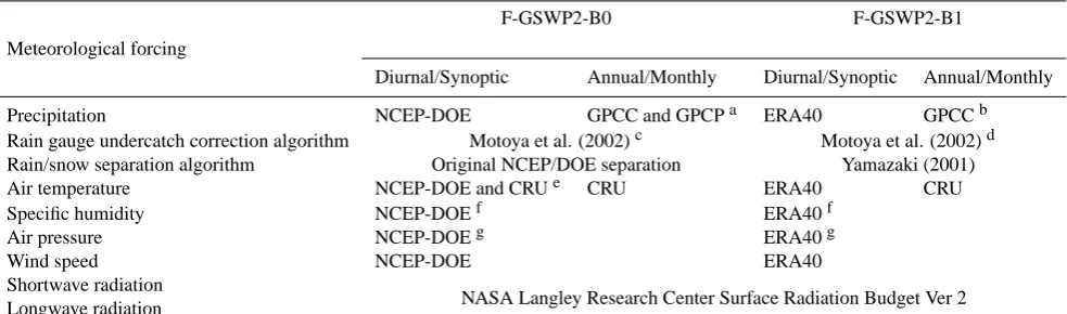
Table 1. Differences in meteorological forcing inputs between F-GSWP2-B0 and F-GSWP2-B1.
Meteorological forcing
F-GSWP2-B0 F-GSWP2-B1
Diurnal/Synoptic Annual/Monthly Diurnal/Synoptic Annual/Monthly
Precipitation NCEP-DOE GPCC and GPCPa ERA40 GPCCb
Rain gauge undercatch correction algorithm Motoya et al. (2002)c Motoya et al. (2002)d
Rain/snow separation algorithm Original NCEP/DOE separation Yamazaki (2001)
Air temperature NCEP-DOE and CRUe CRU ERA40 CRU
Specific humidity NCEP-DOEf ERA40f
Air pressure NCEP-DOEg ERA40g
Wind speed NCEP-DOE ERA40
Shortwave radiation
NASA Langley Research Center Surface Radiation Budget Ver 2 Longwave radiation
a GPCC was used for grids where rain gauges were densely located, whereas GPCP was used for grids where they were sparsely located. b GPCP was not used.
c The algorithm of Motoya et al. (2002) and NCEP-DOE wind speed at the height of 10 m were used.
d The algorithm of Motoya et al. (2002) and ERA40 wind speed at the height of 2 m (originally 10 m) were used. e Daily maximum and minimum temperature changes were scaled linearly by CRU data.
f Adjusted to corrected air temperature so that the relative humidity of the original reanalysis was conserved. g Adjusted to ISLSCP2 elevation.
0 500 1000 1500 2000
0 500 1000 1500 2000
Precipitation [mm/yr]
0 500 1000 1500 2000
0 500 1000 1500 2000 0
5 10
0 5 10
Wind speed at the height of 10m [m/s]
0 5 10
0 5 10
0 5 10
0 5 10 F−GSWP2−B0
0 5 10
0 5 10
0 500 1000 1500 2000
0 500 1000 1500 2000
Precipitation [mm/yr]
0 500 1000 1500 2000
0 500 1000 1500 2000 0
5 10
0 5 10
Wind speed at the height of 10m [m/s]
0 5 10
0 5 10
0 5 10
0 5 10
F−GSWP2−B1
0 5 10
0 5 10
0 500 1000 1500 2000
0 500 1000 1500 2000
Precipitation [mm/yr]
0 500 1000 1500 2000
0 500 1000 1500 2000 0
5 10
0 5 10
Wind speed at the height of 10m [m/s]
0 5 10
0 5 10
0 5 10
0 5 10
CRU
0 5 10
0 5 10
S60 S30 EQ N30 N60 N90
0 5 10
0 5 10
Fig. 1. Comparison of zonal mean wind speed and precipitation.
The NCEP-DOE reanalysis was corrected linearly to match the monthly mean values to the observation-based data. For the precipitation data, an algorithm for the gauge correction of wind-caused undercatch was applied to the rainfall and snowfall input data (Motoya et al., 2002). The methodology for producing these components has been described in de-tail by Zhao and Dirmeyer (2003), and a short description is provided in Appendix A.
To revisit the findings of Decharme and Douville (2006), the global zonal mean distributions of wind speed and pre-cipitation of F-GSWP2-B0 are provided (Fig. 1). As a yard-stick, the mean 1961–1990 global observation-based data of
the Climate Research Unit at the University of East Anglia (CRU; New et al., 1999) are provided for wind speed and precipitation. The precipitation of F-GSWP2-B0 is clearly larger than that of the CRU at middle to high latitudes, but smaller at low latitudes. One possible cause of the large pre-cipitation of F-GSWP2-B0 is its wind speed, which is much higher than that of the CRU except at low latitudes. Mo-toya et al.’s (2002) undercatch correction is correlated with wind speed (see Appendix A), especially in regions at high latitudes in which precipitation is dominated by snow. More-over, we obtained the original source program code that was used to produce F-GSWP2-B0 precipitation data and found that wind speed at a height of 10 m was used, whereas Mo-toya et al.’s (2002) algorithm expects a height of 2 m. This is another cause of overcorrection in F-GSWP2-B0 precipita-tion data because wind speed is stronger at higher altitudes.
[image:4.595.53.285.381.530.2]around the world and found better agreement with ERA40 than with NCEP-DOE. Because daily and diurnal variation in the GSWP2 meteorological forcing inputs is dependent on the reanalysis data, we substituted the ERA40 data for the NCEP-DOE data.
The wind speed of F-GSWP2-B1 is more similar to that of the CRU than the F-GSWP2-B0, but it is smaller than that of the CRU at southern low latitudes (Fig. 1). For precip-itation, F-GSWP2-B1 has greater precipitation at latitudes higher than 50◦N in the Northern Hemisphere and higher than 35◦S in the Southern Hemisphere because of the under-catch correction, but the difference from the CRU is much smaller than that from the F-GSWP2-B0 (Fig. 1).
3 Model
3.1 Land surface hydrology module
A land surface hydrology module calculates the energy and water budget, including snow, on the land surface from the forcing data. This module is based on a bucket model (Man-abe, 1969; Robock et al., 1995), but differs from the original formulation in the following three aspects. First, soil tem-perature is calculated using the force restore method (Bhum-ralkar, 1975; Deardorff, 1978) to simulate the diurnal cycle of surface temperature reasonably using three-hourly meteo-rological forcing inputs. Second, a simple subsurface runoff parameterization is added to the model. Third, two indepen-dent land surface conditions can be simulated within a single grid that is intended to separate irrigated cropland from other land types. The bucket model is simple, but is still widely used in current global water hydrological studies. Soil mois-ture is expressed as a single-layer bucket 15 cm deep for all soil and vegetation types. When the bucket is empty, soil moisture is at the wilting point; when the bucket is full, soil moisture is at field capacity. Evapotranspiration is expressed as a function of potential evapotranspiration and soil mois-ture. In the original bucket model, runoff is generated only when the bucket is overfilled, but we used a “leaky bucket” formulation in which soil moisture drains continuously. Po-tential evapotranspiration and snowmelt are calculated from the surface energy balance. A detailed description of this module can be found in Appendix B.
At first, the parameters of the land surface hydrology mod-ule were set as globally uniform (Appendix B). However, there was substantial regional bias in runoff and streamflow simulations. Therefore, we set the parameters of the land surface hydrology modules for four climatic zones from an analysis of energy and water constraint (Appendix C). Here-after, only the results obtained using the modified parameters are shown for clarity of discussion.
3.2 River routing module
The river module is identical to the Total Runoff Integrating Pathways model (TRIP; Oki and Sud, 1998; Oki et al., 1999). The module has a digital river map with a spatial resolu-tion of 1◦×1◦(the land–sea mask is identical to the GSWP2 meteorological forcing input) and a flow velocity fixed at 0.5 m s−1. The module accumulates runoff calculated by the land surface hydrology module and outputs streamflow. This module does not deal with lakes or swamps, human-made reservoir operation, diversion or withdrawal, or evaporation loss from water surfaces. Human-made reservoir operation and withdrawal are modeled in the respective modules. 3.3 Crop growth module
We coded a crop growth module with reference to the Soil Water Integrated Model (SWIM; Krysanova et al., 1998, 2000). The SWIM model is an eco-hydrological model for regional impact assessments in mesoscale watersheds (100– 10 000 km2). The model integrates hydrology, vegetation, erosion, and nitrogen dynamics at the watershed scale. We used only the formulation and parameters of crop vegetation. The SWIM model can deal with more than 50 types of crops. For 18 of these crop types, Leff et al. (2004) provided the global distribution of the areal proportion at a 0.5◦×0.5◦ spa-tial resolution. The remaining crops were simulated using a generic parameter set. Because the SWIM model is a descen-dant of the Erosion Productivity Impact Calculator (EPIC) model (Williams, 1995) and the Soil Water Assessment Tool (SWAT) model (Neitsch et al., 2002), the formulation and parameters of the crop module are quite similar to those of the earlier models (Appendix D).
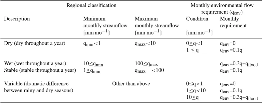
Table 2. Environmental flow requirements of the environmental flow requirement module of the integrated model; q indicates monthly
runoff.
Regional classification Monthly environmental flow
requirement (qenv)
Description Minimum Maximum Condition Monthly
monthly streamflow monthly streamflow requirement
[mm mo−1] [mm mo−1] [mm mo−1]
Dry (dry throughout a year) qmin<1 qmax<10 0≤q<1 qenv=0 1≤q qenv=0.1q
Wet (wet throughout a year) 10≤qmin 100≤qmax qenv=0.3q+qflood
Stable (stable throughout a year) 1≤qmin qmax <100 qenv=0.1q
Variable (dramatic difference Other than above 0≤q<1 qenv=0
between rainy and dry seasons) 1≤q<10 qenv=0.1q
10≤q qenv=0.3q+qflood
A simplified cropping pattern was assumed because of limited detailed information on global cropping practices. We assumed that the same crop species was planted in both irrigated and nonirrigated croplands. The global distribu-tion of crop species was obtained from Leff et al. (2004). To further simplify the simulation, only information on pri-mary and secondary crop types in terms of the cultivated area reported by Leff et al. (2004) was used. We then assumed that the primary crop was cultivated as the first crop, and the secondary crop was cultivated as the second crop. The crop intensity of irrigated cropland (the areal proportion of cultivated area to the total irrigated area) was obtained from D¨oll and Siebert (2002). According to their estimation, crop intensity varied from 0.8 (i.e., on average, 80% of the to-tal irrigated cropland is used) in parts of the former USSR, Baltic states, and Belarus to 1.5 in eastern Asia, Oceania, and Japan. For the former group of countries, we assumed that only 80% of the irrigated land was cultivated for the first crop and that no second crop was planted. For the latter group, we assumed 100% cultivation for the first crop and 50% for the second crop.
3.4 Reservoir operation module
In the global river map of the river routing module, the 452 largest reservoirs with storage capacity>109m3each world-wide were geo-referenced, and available reservoir informa-tion (e.g., name, purposes in order of priority, and storage capacity) was compiled (Hanasaki et al., 2006). The total storage capacity of these 452 reservoirs was 4140 km3, ac-counting for approximately 60% of the total reservoir storage capacity in the world (ICOLD, 1998). The reservoir opera-tion module set operating rules for individual reservoirs. For reservoirs for which the primary purpose was not irrigation water supply, the reservoir operating rule was set to minimize
interannual and subannual streamflow variation (i.e., storage capacity and inflow). For reservoirs for which irrigation wa-ter supply was the primary purpose, daily release from the reservoir was proportional to the irrigation water requirement in the lower reaches (Appendix E).
3.5 Environmental flow requirement module
We estimated a monthly environmental flow requirement us-ing the algorithm of Shirakawa (2004, 2005). Because both reports by Shirakawa were published in Japanese, we first describe Shirakawa’s methodology. First, using the 10-year mean monthly gridded streamflow data simulated by the land surface hydrology module and the river routing module, all grids were classified into four regions following specific cri-teria (Table 2). The environmental flow requirement con-sisted of two factors: the base requirement, which was the minimum streamflow in the channel; and the perturbation re-quirement, which allowed flush streamflow in the rainy sea-son. The perturbation requirement was 10% of the mean monthly streamflow and should occur for 2–3 days. How-ever, considering the spatiotemporal resolution of our study, the perturbation requirement was not implemented; instead, an allocated amount was simply added to the base require-ment (Appendix F).
theory regarding environmental flow requirements. Indeed, value judgments are largely influenced by regional welfare and culture. However, because of limited information re-garding global applicability, the algorithm only accounted for natural hydrological conditions; cultural and economic perspectives were not considered.
3.6 Anthropogenic water withdrawal module
The anthropogenic water withdrawal module withdraws the amount of consumptive water use for domestic, industrial, and agricultural purposes from river channels in that order at each simulation grid cell. This module plays an impor-tant role in coupling water fluxes among the land surface hy-drology, river routing, crop growth, and environmental flow requirement modules.
Domestic and industrial water use was not estimated by the integrated model. Instead, this information was ob-tained from the AQUASTAT database (Food and Agricul-ture Organization, 2007). The AQUASTAT database pro-vides statistics-based national water withdrawal data for do-mestic, industrial, and agricultural sectors. These data were converted to gridded data by weighting the population dis-tribution and national boundary information provided by the Center for International Earth Science Information Network (CIESIN) of Columbia University and Centro Internacional de Agricultura Tropical (CIAT; 2005). The values were then converted to the consumptive amount, which is the evapo-rated portion of the total withdrawal. We used 0.10 for do-mestic water and 0.15 for industrial water, from the study of Shiklomanov (2000). Seasonal variation was not taken into account for these water uses. For future simulations, projec-tions of other studies such as that by Shen et al. (2008) will be used.
When streamflow was less than the total water demand, streamflow except for the share of environmental flow, was withdrawn. Withdrawn irrigation water was added to the soil moisture in irrigated areas, and domestic and indus-trial waters were removed from the system. This latter pro-cess was an exception to the closure of the energy and wa-ter balances; however, the sum of consumptive domestic and industrial water was 132.4 km3yr−1 in 1995 (Shiklo-manov, 2000). This amount was two orders of magnitude less than global runoff and evaporation (40 000 km3yr−1and 71 000 km3yr−1, respectively; Baumgartner and Reichel, 1975) and was thus judged to be negligible.
180˚ 210˚ 240˚ 270˚ 300˚ 330˚ 0˚ 30˚ 60˚ 90˚ 120˚ 150˚ 180˚
−60˚ −30˚ 0˚ 30˚ 60˚ 90˚
180˚ 210˚ 240˚ 270˚ 300˚ 330˚ 0˚ 30˚ 60˚ 90˚ 120˚ 150˚ 180˚
−60˚ −30˚ 0˚ 30˚ 60˚ 90˚
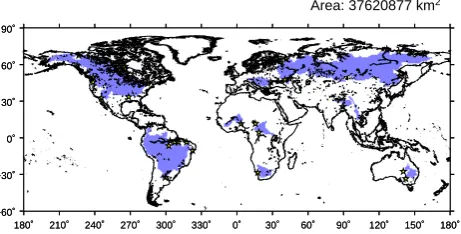
[image:7.595.313.544.66.183.2]Area: 37620877 km2
Fig. 2. Comparison of zonal mean wind speed and precipitation.
Distribution of river gauging stations (stars). The shaded areas rep-resent catchments.
4 Validation of the simulated global hydrological cycle
4.1 Validation methodology
To confirm that the global hydrological cycle was properly simulated using our meteorological forcing data sets and the land surface hydrology module, simulated runoff and stream-flow were validated by comparison with observations and earlier studies. First, the land surface hydrology module and the river routing module were coupled, and a global natu-ral hydrological simulation was conducted using two meteo-rological forcing data sets. Hereafter the runoff/streamflow product obtained using F-GSWP2-B1 is called R-GSWP2-B1 (R stands for runoff; the forcing data were F-GSWP2-R-GSWP2-B1) and that using F-GSWP2-B0 is called R-GSWP2-B0.
Table 3. Earlier studies of global runoff estimation.
Data Period Time Space Source Output Param. Simulation Precipitation
Corr.1 Tune2 time step
R-GSWP2-B1 1986–1995 Daily 1.0◦×1.0◦ This study 3 h Rudolf et al., 1994
R-N01 1980–1993 Daily 1.0◦×1.0◦ Nijssen et al., 2001 Y Day Huffman et al., 1997
R-F02 Clim. Monthly 0.5◦×0.5◦ Fekete et al., 2002 Y Month Willmott and coauthors3
R-D03 1901–1995 Monthly 0.5◦×0.5◦ D¨oll et al., 2003 Y Y Day New et al., 2000
R-BR75 Clim. Annually 5.0◦zonal Baumgartner and Year Original
Reichel, 1975
1. Output runoff data were corrected so that simulated long-term mean annual streamflow agreed with the observations. 2. Model parameter was tuned at specific river basins.
3. http://climate.geog.udel.edu/∼climate/index.shtml, last access: 3 May 2008.
0 100 200 300 400 500 600 700 800 900 1000 0 100 200 300 400 500 600 700 800 900 1000 0 100 200 300 400 500 600 700 800 900 1000 0 100 200 300 400 500 600 700 800 900 1000 0 100 200 300 400 500 600 700 800 900 1000 0 100 200 300 400 500 600 700 800 900 1000 0 100 200 300 400 500 600 700 800 900 1000 0 100 200 300 400 500 600 700 800 900 1000 0 100 200 300 400 500 600 700 800 900 1000 0 100 200 300 400 500 600 700 800 900 1000 0 100 200 300 400 500 600 700 800 900 1000 0 100 200 300 400 500 600 700 800 900 1000 0 100 200 300 400 500 600 700 800 900 1000 0 100 200 300 400 500 600 700 800 900 1000 0 100 200 300 400 500 600 700 800 900 1000 0 100 200 300 400 500 600 700 800 900 1000 0 100 200 300 400 500 600 700 800 900 1000 0 100 200 300 400 500 600 700 800 900 1000 0 100 200 300 400 500 600 700 800 900 1000 0 100 200 300 400 500 600 700 800 900 1000 0 100 200 300 400 500 600 700 800 900 1000 0 100 200 300 400 500 600 700 800 900 1000 0 100 200 300 400 500 600 700 800 900 1000 0 100 200 300 400 500 600 700 800 900 1000 0 100 200 300 400 500 600 700 800 900 1000 0 100 200 300 400 500 600 700 800 900 1000 0 100 200 300 400 500 600 700 800 900 1000 0 100 200 300 400 500 600 700 800 900 1000 0 100 200 300 400 500 600 700 800 900 1000 0 100 200 300 400 500 600 700 800 900 1000 0 100 200 300 400 500 600 700 800 900 1000 0 100 200 300 400 500 600 700 800 900 1000 0 100 200 300 400 500 600 700 800 900 1000 0 100 200 300 400 500 600 700 800 900 1000 0 100 200 300 400 500 600 700 800 900 1000 R−GSWP2−B0 0 100 200 300 400 500 600 700 800 900 1000 0 100 200 300 400 500 600 700 800 900 1000 0 100 200 300 400 500 600 700 800 900 1000 R−GSWP2−B1 0 100 200 300 400 500 600 700 800 900 1000 0 100 200 300 400 500 600 700 800 900 1000 0 100 200 300 400 500 600 700 800 900 1000 R−N01 0 100 200 300 400 500 600 700 800 900 1000 Runoff[mm/yr]
Asia Europe Africa N_Ame S_Ame Oceania Globe
0 100 200 300 400 500 600 700 800 900 1000
Fig. 3. Mean annual runoff for each continent. Gray shading
in-dicates the range of runoff estimated by earlier observation-based studies (Baumgartner and Reichel, 1975; Fekete, 2002; D¨oll et al., 2003). If the bar height lies within the shaded region, then runoff can be considered plausible
generally regarded as the best available data and have been cited extensively by earlier studies. Our focus here was to examine how closely our results fit these previous data.
Three gridded global runoff data sets of earlier studies were also routed using the river routing module. R-D03, R-F02, and R-N01 were re-gridded so that they matched both the land/sea distribution and the spatial resolution of F-GSWP2-B1. For R-N01 data, which have 2.0◦×2.0◦ resolu-tion, identical runoff was allocated to four 1.0◦×1.0◦grids. For R-F02 and R-D03 data, which have 0.5◦×0.5◦ resolu-tion, the runoff of four grids was aggregated into one grid. The Antarctic, Greenland, and lake grids (e.g., Great Lakes in USA and Canada) were excluded from analysis. Finally, simulated streamflow was obtained at 32 river gauging sta-tions.
[image:8.595.52.282.251.398.2]4.2 Continental runoff
Figure 3 shows simulated runoff at the continental scale for three runoff products (GSWP2-B0, GSWP2-B1, R-N01). R-GSWP2-B1 was within the plausible range (i.e., the runoff range of the observation-based data sets F02, R-D03, and R-BR75) of runoff in Asia, North America, South America, Oceania, and the globe (Fig. 3). In Europe and Africa, it exceeded plausible values by 27% and 10%, re-spectively. In contrast, R-GSWP2-B0 was the largest among the data sets. In this case, simulated runoff greatly exceeded the range of the three earlier projections in Europe and North America.
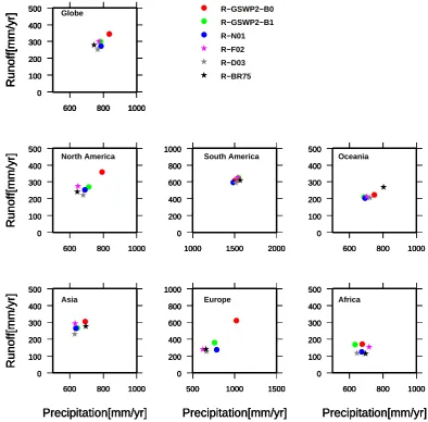
Earlier studies showed a linear relationship between pre-cipitation and runoff (Fig. 4). The observation-based data sets, namely R-F02, R-D03, and R-BR75, gave similar re-sults, indicating that they are consistent in precipitation and runoff. This linear relationship emphasizes precipitation as the dominant factor in the production of continental runoff. Except for Europe and Africa, R-GSWP2-B1 precipitation is similar to that of R-F02, R-D03, and R-BR75; consequently, the projected runoff is also similar. Except for a few cases, R-GSWP2-B0 projects into the upper right, which means larger input precipitation was used and larger runoff was produced compared to earlier studies. The hydrological simulation of the land surface hydrology module shows better performance with F-GSWP2-B1 than with F-GSWP2-B0, mainly because its precipitation input is plausible.
The large precipitation in Europe from F-GSWP2-B1 pro-duced large runoff (Fig. 4). This large precipitation was caused by the rain gauge undercatch correction applied to F-GSWP2-B1 precipitation forcing inputs. Even larger precipi-tation (similar to F-GSWP2-B1) was given; R-N01 is similar to that of R-F02, R-D03, and R-BR75. This is primarily a re-sult of the basin-level hydrological parameter tuning applied to the model used for R-N01.
0 100 200 300 400 500
Runoff[mm/yr]
600 800 1000
Precipitation[mm/yr]
0 200 400 600 800 1000500 1000 1500
Precipitation[mm/yr]
0 100 200 300 400 500600 800 1000
Precipitation[mm/yr]
0 100 200 300 400 500Runoff[mm/yr]
600 800 1000 0 200 400 600 800 1000
1000 1500 2000 0 100 200 300 400 500
600 800 1000 0 100 200 300 400 500
Runoff[mm/yr]
600 800 1000 0 100 200 300 400 500
Runoff[mm/yr]
600 800 1000
0 100 200 300 400 500
Runoff[mm/yr]
600 800 1000
Precipitation[mm/yr]
0 200 400 600 800 1000500 1000 1500
Precipitation[mm/yr]
0 100 200 300 400 500600 800 1000
Precipitation[mm/yr]
0 100 200 300 400 500Runoff[mm/yr]
600 800 1000 0 200 400 600 800 1000
1000 1500 2000 0 100 200 300 400 500
600 800 1000 0 100 200 300 400 500
Runoff[mm/yr]
600 800 1000 0 100 200 300 400 500
Runoff[mm/yr]
600 800 1000 Globe
Asia Europe Africa
North America South America Oceania
R−GSWP2−B0 R−GSWP2−B1 R−N01 R−F02 R−D03 R−BR75 0 100 200 300 400 500
Runoff[mm/yr]
[image:9.595.98.493.79.467.2]600 800 1000
Fig. 4. The relationship between runoff and precipitation. Stars indicate observation-based studies.
attributable to factors other than precipitation, mainly low wind speed. The zonal mean runoff distribution in Africa indicates that the runoff at lower latitudes exceeds that of previous studies, although there is no significant difference in zonal mean precipitation among the earlier studies and F-GSWP2-B1 (not shown). The F-F-GSWP2-B1 wind speed is low at low latitudes, and evaporation is considered to be re-stricted (Fig. 1). In the land surface hydrology module, evap-oration is basically correlated with wind speed (Appendix B).
4.3 Runoff in individual basins
The simulated streamflow data sets were validated at 32 major river gauging stations. Using the simulated and ob-served data, the normalized bias of mean annual streamflow (NBIAS), the difference in the arrival of peak streamflow
(PEAK), and the correlation coefficient (CC) of variation in annual streamflow were calculated as follows:
NBIAS=(s−o)
o (1)
PEAK=
P1995
y=1986
my,sim−my,obs
10 (2)
CC=
P1995
y=1986 sy−s oy−o
q P1995
y=1986 sy−s
2qP1995
y=1986 oy−o
2 (3)
where o is the mean annual observed streamflow (calcu-lated from available records between 1986 and 1995), s is the mean annual simulated streamflow (calculated for months in which o was available), my,sim is the month in
NBIAS
R−GSWP2−B1 R−N01
R−F02 R−D03
−1.0 −0.5 −0.2 0.2 0.5 1.0 100.0
PEAK
R−GSWP2−B1 R−N01
R−F02 R−D03
0 1 2 3 6
CC
R−GSWP2−B1 R−N01
R−F02 R−D03
[image:10.595.56.278.62.654.2]−1.0 −0.8 −0.6 0.6 0.8 1.0
Fig. 5. Validation results for 32 river basins. (a) Normalized bias
of mean annual runoff (NBIAS). (b) Delay in the arrival of peak streamflow (PEAK). R-N01, R-F02, and R-D03 are not shown be-cause their data are monthly and thus too coarse for routing. (c) Cor-relation coefficient of annual streamflow (CC). R-F02 are not shown because their simulation periods were one climatological year.
the monthly simulated streamflow, and oy is the monthly
observed streamflow. The subscript y indicates the year. NBIAS is calculated to evaluate the simulated water balance in basins, PEAK to evaluate the timing of streamflow peaks in basins, and CC to evaluate the interannual variation in streamflow. Because lakes and reservoirs affect PEAK and CC considerably, five river basins, namely, the Don, Parana, Sao Fransisco, St. Lawrence, and Nelson, were excluded from calculations of PEAK and CC. R-BR75 was excluded because it reports only zonal mean runoff data. First, we ex-amine NBIAS (Fig. 5a). For R-GSWP2-B1, NBIAS is less than±50%, except for some river basins in Africa and north-eastern South America. These basins are located in semi-arid to arid climatic zones, and runoff was significantly overes-timated in these basins (>50% and sometimes >100% of the mean annual difference). The runoff of these basins was commonly overestimated in most of the earlier studies. R-N01 reproduced runoff fairly well, especially for river basins in Siberia. R-F02 and R-D03 showed even better agreement, although these two results are not surprising because the data sets were scaled so that simulated streamflow matched long-term mean annual streamflow. There were some basins with errors>20% because the period selected for scaling in these studies may have differed from ours. In the case of R-D03, there might be another reason for this disagreement, namely that a maximum change of 100% was allowed for the cor-rection factor. In contrast, for R-GSWP2-B0, the runoff in a large number of basins in North America, Europe, and west-ern Siberia was significantly overestimated (>50% of ob-served); NBIAS in eastern Siberia (e.g., the Amur River and Lena River) was an exception because the simulated runoff was well reproduced.
Second, we examine PEAK (Fig. 5b). R-GSWP2-B1 re-produced the timing of long-term mean monthly streamflow well. In most of the basins, the error was within±2 mo yr−1. The results of the earlier studies for N01, F02, and R-D03 are not shown because their runoff data are at monthly intervals and thus are too coarse for a discussion of monthly peak flow.
Third, we examine CC (Fig. 5c). Because the simulation period of R-F02 involved 1 year of climatological informa-tion, the CCs for R-F02 are not shown. As in Fig. 4, simu-lated runoff (or streamflow) was strongly corresimu-lated with in-put precipitation. Because precipitation in the earlier studies was based on ground observations, it seems that the annual variation in simulated runoff agrees well with the observa-tions.
0 1 0 1 2 3 4 0 1 2 3 4 CHARI 0 1 2 3 4 0 1 2 3 4 0 1 2 3 4 UBANGI 0 1 2 3 4 0 1 2 3 4 0 1 2 3 4 MEKONG 0 1 2 3 4 0 1 2 3 4 0 1 2 3 4 BRAHMAPUTRA 0 1 2 3 4 0 1 2 3 4 0 1 2 3 4 LENA 0 1 2 3 4 0 1 2 3 4 0 1 2 3 4 AMUR 0 1 2 3 4 0 1 2 3 4 0 1 2 3 4 YENISEI 0 1 2 3 4 0 1 2 3 4 0 1 2 3 4 OB 0 1 2 3 4 0 1 2 3 4 0 1 2 3 4 YANA 0 1 2 3 4 0 1 2 3 4 0 1 2 3 4 INDIGIRKA 0 1 2 3 4
86 87 88 89 90 91 92 93 94 95
0 1 2 3 4 0 1 2 3 4 0 1 2 3 4 KOLYMA 0 1 2 3 4 0 1 2 3 4 0 1 2 3 4 MAGDALENA 0 1 2 3 4 0 1 2 3 4 0 1 2 3 4 PARANA 0 1 2 3 4 0 1 2 3 4 0 1 2 3 4 AMAZONAS 0 1 2 3 4 0 1 2 3 4 0 1 2 3 4 RIO_TAPAJOS 0 1 2 3 4 0 1 2 3 4 0 1 2 3 4 XINGU 0 1 2 3 4 0 1 2 3 4 0 1 2 3 4 TOCANTINS 0 1 2 3 4 0 1 2 3 4 0 1 2 3 4 RIO_PARNAIBA 0 1 2 3 4 0 1 2 3 4 0 1 2 3 4 SAO_FRANCISCO 0 1 2 3 4 0 1 2 3 4 0 1 2 3 4 YUKON_RIVER 0 1 2 3 4
86 87 88 89 90 91 92 93 94 95
0 1 2 3 4 0 1 2 3 4 0 1 2 3 4 COLUMBIA_RIVER 0 1 2 3 4 0 1 2 3 4 0 1 2 3 4 MISSISSIPPI_RIVER 0 1 2 3 4 0 1 2 3 4 0 1 2 3 4 ST._LAWRENCE_RIVER 0 1 2 3 4 0 1 2 3 4 0 1 2 3 4 FRASER_RIVER 0 1 2 3 4 0 1 2 3 4 0 1 2 3 4 MACKENZIE_RIVER 0 1 2 3 4 0 1 2 3 4 0 1 2 3 4 NELSON_RIVER 0 1 2 3 4 0 1 2 3 4 0 1 2 3 4 CHURCHILL_RIVER 0 1 2 3 4 0 1 2 3 4 0 1 2 3 4 DANUBE 0 1 2 3 4 0 1 2 3 4 0 1 2 3 4 NORTHERN_DVINASEVERNAYA_DVIN 0 1 2 3 4 0 1 2 3 4 0 1 2 3 4 PECHORA 0 1 2 3 4
86 87 88 89 90 91 92 93 94 95
[image:11.595.73.518.67.366.2]0 1 2 3 4 0 1 2 3 4 0 1 2 3 4 VOLGA 0 1 2 3 4 0 1 2 3 4 0 1 2 3 4 DON 0 1 2 3 4 0 1 2 3 4
Fig. 6. Normalized monthly streamflow at 32 validation basins. Bold solid line, observation; thin solid line, simulation. Monthly streamflow
was normalized so that the mean annual streamflow from 1986 to 1995 (or available records in this period) equaled one.
Table 4. The number of river gauging stations meeting the criteria for the normalized bias of mean annual streamflow (NBIAS), the difference
in the month of arrival of the peak of streamflow [mo yr−1] (PEAK), and the correlation coefficient of interannual streamflow variation (CC).
Data –0.5≤BIAS≤0.5 PEAK≤2.0 0.6≤CC –0.2≤BIAS≤0.2 PEAK≤1.0 0.8≤CC
R-GSWP2-B0 16 25 21 7 19 10
R-GSWP2-B1 24 25 22 14 16 13
R-N01 22 – 22 14 – 15
R-F02 30 – – 25 – –
R-D03 27 – 22 19 – 13
Total validation basins 32 27 27 32 27 27
and was similar to R-N01; however, only 14 of the 32 river basins met the criteria. R-D03 was generated so that long-term mean annual discharges matched, but not all river basins agreed with observations within±20% error. The number of basins that met the criteria of PEAK and CC were 16 and 13 of the 32 river basins, respectively. The performance of CC was quite similar among GSWP2-B1, N01, and R-D03. Our results indicate that it is still a challenge for global hydrology models to simulate annual river discharge year by year. We changed the set of thresholds to±50% for NBIAS,
±2 mo for PEAK, and 0.6 for CC (Table 4). In this case, NBIAS, PEAK, and CC of R-GSWP2-B1 agreed with the
[image:11.595.82.516.450.540.2]The goal of the integrated model was to assess the suban-nual distribution of water availability and water use. Figure 6 shows the normalized monthly streamflow of R-GSWP2-B1 and observations at 32 validation basins from 1986 to 1995. The monthly streamflow was normalized so that the mean annual streamflow from 1986 to 1995 equaled one. It is clear that significant seasonality occurs in many basins; these ex-hibited more than three times the mean annual streamflow for only a few months per year, and in the remaining months, streamflow was far less than one. The results indicate that we can move forward to assess the seasonal variability in global water resources.
5 Summary
To assess global water resources taking into account suban-nual variability, we developed an integrated model that com-prised six modules. We revisited the original GSWP2 me-teorological forcing input (F-GSWP2-B0) and developed an improved meteorological forcing data set (F-GSWP2-B1). We then presented the six modules: land surface hydrol-ogy, river routing, crop growth, reservoir operation, envi-ronmental flow requirement estimation, and anthropogenic water withdrawal. Finally, simulated runoff and streamflow were validated by comparison with observations and earlier works. The performance was similar to the best available precedent studies with closure of energy and water. This result indicates the validity of the model and input meteo-rological forcing. In our companion paper, we present the model application. Using the daily simulation outputs, we conduct global water resource assessments, focusing on sub-annual variation in water availability and water use.
Appendix A
F-GSWP2-B0 meteorological forcing input
The F-GSWP2-B0 meteorological forcing input is a hy-brid product of NCEP-DOE reanalysis (Kanamitsu et al., 2002) and various observation-based monthly gridded meteorological data. The air temperature input is a hybrid product of NCEP-DOE reanalysis (Kanamitsu et al., 2002) and observation-based monthly temperature data of the Cli-mate Research Unit at University of East Anglia (CRU; New et al., 2000). First, the air temperature from the origi-nal NCEP-DOE reaorigi-nalysis was re-gridded from the native 1.9◦×1.9◦resolution to the ISLSCP2 required 1◦×1◦ reso-lution and processed from hourly data to three-hourly data (Zhao and Dirmeyer, 2003). The air temperature of the CRU was scaled to adjust for the altitude difference between the CRU grid and the ISLSCP2 mean altitude. The NCEP-DOE reanalyses were linearly scaled so that the monthly mean val-ues were identical to the CRU valval-ues. The air temperature
data were linearly scaled again so that the diurnal tempera-ture range for each month was identical to that of the CRU. In this way, the air temperature of NCEP-DOE was linearly scaled so that the monthly maximum, minimum, and mean air temperatures were identical to those of the CRU. The daily and three-hourly variations were not corrected; they were determined by the NCEP-DOE reanalysis.
For specific humidity and air pressure, the original NCEP-DOE data were corrected so that they were consistent with the altitude of ISLSCP2 and air temperature. For wind speed, NCEP-DOE data were used without any correction. For longwave and shortwave downward radiation, three-hourly Surface Radiation Budget (SRB) data produced at the NASA/Langley Research Center were used (Stackhouse et al., 2000).
The precipitation forcing input is also a hybrid product of the NCEP-DOE reanalysis, the global observational data set GPCC (Rudolf et al., 1994), and the GPCP (Huffman et al., 1997). GPCC data were used for grids where rain gauges were densely located, and GPCP data were used for grids where they were sparsely located. For precipitation data, an algorithm for rain gauge correction for wind-caused under-catch was applied to the rainfall and snowfall input data set (Motoya et al., 2002). In Motoya et al.’s (2002) algorithm, the catchment ratio of snowfall (CRsnow)and that of rainfall
(CRrain)are expressed as follows:
CRsnow=
αexp(bU ) raingauge type known 50.0 exp(−0.182U )+50.0 exp(−0.112U )raingauge type unknown (A1)
CRrain=100.0−1.51U−0.21U2 (A2)
whereUis wind speed at a height of 2 m, andaandbare pa-rameters from Sevruk (1982) and Sevruk and Hamon (1984) that depend on the rain gauge type. The corrected rainfall (Rainf) and snowfall (Snowf) are expressed as
Snowf=Snowforg/CRsnow×100
Rainf=Rainforg/CRrain×100.
(A3) where Rainforg and Snowforg are the original rainfall and
snowfall, respectively. These equations indicate that stronger wind requires a stronger correction and that snowfall requires a stronger correction than rainfall. For example, if the wind speed is 5 m s−1and the rain gauge type is unknown,CRsnow
is 48.7% andCRrainis 87.2%.
The revised meteorological forcing F-GSWP2-B1 was prepared using the same methodology, but different data sets (see Table 1).
Appendix B
The land surface hydrology module
B1 Albedo
the GSWP2 standard monthly land use data set and included plant phenological aspects. The snow surface albedo (αsnow)
varied according to the surface temperature (Ts)as follows
(Robock et al., 1995):
αsnow=
αmax TS≤Tcrit
{αmax×(Tmelt−TS)+αmin×(TS−Tcrit)}/ (Tmelt−Tcrit) Tcrit≤TS≤Tmelt
αmin Tmelt≤TS
(B1) whereαmaxis the maximum snow albedo, fixed at 0.60;αmin
is the minimum snow albedo, fixed at 0.45;Tcritis the critical
temperature (263.15 K); andTmeltis the melting point of ice
(273.15 K). The surface albedo was expressed as
α=
αsnow 20≤SWE
αsoil+ √
0.05·SWE×(αsnow−αsoil) 0<SWE≤20
αsoil SWE=0
(B2)
where SWE is the snow water equivalent [kg m−2]. B2 Sensible heat and latent heat
Potential evaporationEP [kg m−2s−1] was expressed as
EP(TS)=ρCDU (qSAT(TS)−qa) (B3)
where ρ is the density of air [kg m−3], CD is the bulk
transfer coefficient (0.003), U is the wind speed [m s−1], qSAT(TS)is the saturated specific humidity at surface
tem-perature [kg kg−1], andqais the specific humidity [kg kg−1].
Evaporation from a surface (E)was expressed as
E=βEP(TS) (B4)
where β=
1 0.75Wf≤W
W/Wc W <0.75Wf (B5)
whereW is the soil water content [kg m−2] andWf is the
soil water content at field capacity, which was fixed at 150 [kg m−2]. The sensible heat flux (H )is expressed as
H=Cp∗ρCDU (TS−Ta) (B6)
whereCp∗is the specific heat of air [1005 J kg−1K−1] andTa
is the air temperature [K]. B3 Energy balance
The energy balance was expressed as
(1−α)SW↓+LW↓=σ TS4+ιE+H+G (B7) where SW↓ is the downward shortwave radiation, LW↓ is the downward longwave radiation, σ is the Stefan-Boltzmann constant, ι is the latent heat [2.45×10⁶J kg−1], andGis the soil heat flux. The original bucket model (Man-abe, 1969) does not have soil heat capacity or soil heat flux
because it was not designed to simulate diurnal cycles; how-ever, the meteorological forcing input of GSWP2 is three-hourly. We added the force restore method (Bhumralkar, 1975; Deardorff, 1978) to simulate the surface temperature:
Cs∂T∂tS=(1−α) S↓+L↓−σ Ts4−ιE−H−ωCs(TS−Td)
Cd∂T∂td=(1−α) S↓+L↓−σ Ts4−ιE−H
(B8) whereCs is the surface heat capacity, Cd is the deep soil
heat capacity (Cd=
√
365CS[J m−2K−1]), andωis the
angu-lar velocity
(ω=2π24·60·60[s−1]).
B4 Snow and soil water balance The snow balance was expressed as
dSWE
dt =Snowf−Qsm−Qsub (B9)
where SWE is the snow water equivalent [kg m−2], Snowf is the snowfall rate [kg m−2s−1],Qsmis the snow melt rate
[kg m−2s−1], andQsbis the sublimation rate [kg m−2s−1].
With a snow-covered surface, soil moisture does not change through precipitation or evaporation. The soil water balance was expressed as follows:
dW
dt =Rainf+Qsm−E−Qs−Qsb (B10) whereQs is the surface runoff and Qsb is the subsurface
runoff [kg m−2s−1]. B5 Runoff
Surface runoff (Qs)was generated if the soil water content
exceeded the capacity of soil water (i.e., field capacity): Qs=
W−Wf Wf<W
0 W≤Wf
(B11) Subsurface runoff (Qsb), which was not in the original
bucket model (Manabe, 1969; Robock et al., 1995), was in-corporated to the model as
Qsb=
Wf
τ
W Wf
γ
(B12)
whereQsbis the subsurface runoff [kg m−2s−1] andτ is a
time constant [s]. This equation is similar to the percolation rate of the LPJ model (Gerten et al., 2004). Theγ was set at 2, andτ at 100 days=86400×100 s; both are globally con-stant.
B6 Mosaic


![Table 4. The number of river gauging stations meeting the criteria for the normalized bias of mean annual streamflow (NBIAS), the differencein the month of arrival of the peak of streamflow [mo yr−1] (PEAK), and the correlation coefficient of interannual streamflow variation (CC).](https://thumb-us.123doks.com/thumbv2/123dok_us/9265662.996028/11.595.73.518.67.366/normalized-streamow-differencein-streamow-correlation-coefcient-interannual-streamow.webp)

