www.hydrol-earth-syst-sci.net/15/3679/2011/ doi:10.5194/hess-15-3679-2011
© Author(s) 2011. CC Attribution 3.0 License.
Earth System
Sciences
Spatial variation of the longitudinal dispersion
coefficient in an estuary
D. C. Shaha1, Y.-K. Cho1, M.-T. Kwak1, S. R. Kundu2, and K. T. Jung3
1School of Earth and Environmental Sciences, Research Institute of Oceanography, Seoul National University , Seoul 151-742, Korea
2Department of Oceanography, Chonnam National University, Gwangju 500-757, Korea 3Korea Ocean Research and Development Institute, Ansan 425-600, Korea
Received: 7 June 2011 – Published in Hydrol. Earth Syst. Sci. Discuss.: 12 August 2011 Revised: 1 November 2011 – Accepted: 14 November 2011 – Published: 7 December 2011
Abstract. The effective longitudinal dispersion is a pri-mary tool for determining property distributions in estuar-ies. Most previous studies have examined the longitudinal dispersion coefficient for the average tidal condition. How-ever, information on spatial and temporal variations of this coefficient at low and high tides is scarce. Three years of hydrographic data taken at low and high tide along the main axis of the Sumjin River Estuary (SRE), Korea are used to estimate the spatial and temporal variation of the effective longitudinal dispersion coefficient. The range of the disper-sion coefficient is rather broad at high water slack (HWS) and narrower at low water slack (LWS) because of the differ-ent tidal amplitudes. The spatially varying dispersion coef-ficient has maximal values (>300 m2s−1) near the mouth at high water and decreases gradually upstream, with fluctua-tions. The temporally varying dispersion coefficient appears to be positively correlated with river discharges at both low and high tide. The dispersion varies with the square root of river discharges at HWS and LWS. The dispersive salt fluxes increases with increasing river discharges and decreases with decreasing river discharges at HWS and LWS. Estimation of the numerical values of the effective longitudinal dispersion coefficient in the SRE can be useful for better understand-ing of the distributions of other tracers in the SRE as well as for developing and testing hypotheses about various mixing mechanisms.
Correspondence to: Y.-K. Cho
1 Introduction
Pollutants enter rivers by many routes, including runoff from agricultural land, industrial and municipal wastewater, and tributary discharge. Physical processes such as advective transport and dispersion play key roles in determining the movement and changes in concentration of these contami-nants after they enter a river. Thus, advection and dispersion are fundamental variables for the evaluation of water qual-ity in aquatic systems by conceptual or numerical models (Garcia-Barcina et al., 2006; Ji, 2008). The dispersion co-efficient can be estimated using tracer experiments (Caplow et al., 2003; Ho et al., 2002), but these experiments are logis-tically complex and time consuming. However, the spatial and temporal distribution of salinity in an estuary sampled non-synoptically is a useful indicator of the system’s physi-cal condition because it represents the net effect of numerous complex processes such as the freshwater inflow, tidal range, and degree of turbulence (Lewis and Uncles, 2003; Eaton, 2007).
Dispersive processes in an estuary are usually estimated by a dispersion coefficientDi(x)using salinity as a tracer. Di(x)is usually defined as the ratio of the non-advective
little attention. The tidally averaged salt balance equa-tion has been integrated for high water slack (HWS) and low water slack (LWS) conditions (Savenije, 1989, 2005), which are of greater interest in this study for determining the effective longitudinal dispersion coefficient based on ob-served axial depth-averaged salinity distributions of an estu-ary. Eaton (2007) noted that the spatial distributions of the dispersion coefficient depend strongly on ground-water dis-charge and are most sensitive at LWS.
The numerical values of this longitudinal dispersion co-efficient in estuaries are comparatively difficult to deter-mine and interpret because the motion of solutes in estuar-ies is influenced by river discharge, tidal variations, bed fric-tion, channel topography and density gradients (Guymer and West, 1992; Geyer and Signell, 1992; Vallino and Hopkin-son, 1998; Austin, 2004). The effective longitudinal disper-sion varies temporally and increases with freshwater inflow (Paulson, 1970; Garvine et al., 1992; Dyer, 1997; Austin, 2004). In contrast, theDi(x)values decline with an increase
in tidal range (Lewis and Uncles, 2003). This is because the dispersive action becomes less effective under more turbulent conditions as turbulence generated by strong tidal amplitude effectively reduces the dispersing action of velocity shears (Linden and Simpson, 1988). Moreover, Linden and Simp-son (1988) reported thatDi(x)increases with the horizontal
density gradient and also with the period of the turbulence modulation. The dispersive flux of salt is particularly sensi-tive near the maximum salinity gradient (Lewis and Uncles, 2003).
The Sumjin River discharges into Gwangyang Bay on the south coast of Korea. No information is available about the typical magnitude ofDi(x)along the Sumjin River Estuary
(SRE) or how it changes with variations in freshwater dis-charge, tidal height, and salinity gradient along the SRE. The purpose of this study is to determine the effective longitudi-nal dispersion coefficient at low and high tides in the SRE, which are ultimately responsible for transporting salt up-stream. In addition, the effects of freshwater discharge, tidal height and salinity gradient on the spatially varying longi-tudinal dispersion coefficient are examined. A better knowl-edge of the numerical magnitude of the effective longitudinal dispersion, with some indications of the spatial and temporal variability of this dispersion coefficient, may be useful for developing three dimensional numerical models with more realistic physical fields, which would be helpful for under-standing of biological and chemical distributions in the SRE. The rest of this paper is organized as follows. The study area and data sources are briefly presented in Sect. 2. The methods are described in Sect. 3. The results and discussion are presented in Sect. 4. The conclusions are summarized in Sect. 5.
2 Study site and data
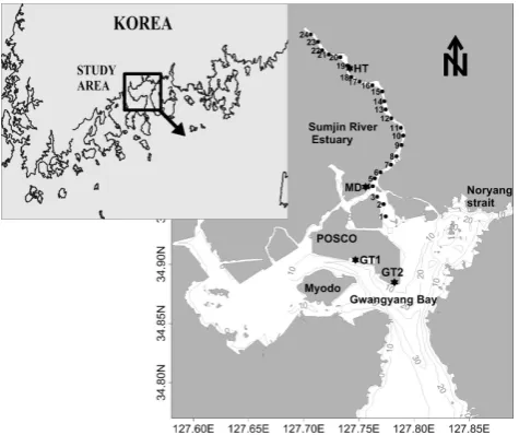
The Sumjin River splits into east and west channels near the Pohang Iron and Steel Company (POSCO) before it en-ters Gwangyang Bay. The bay is connected in the south to the coastal ocean (South Sea) and in the east to Jinjoo Bay through the narrow Noryang Channel (Fig. 1). The cross-sectional area (m2), width (m), and depth (m) of cross-sections of all CTD stations of the SRE were calculated by using Surface Water Modeling System grid generation soft-ware (version 8.1) (Shaha and Cho, 2011). The watershed area of the SRE, including farmland, is almost 4900 km2. Seasonal precipitation and runoff in the Sumjin River basin decrease in spring and winter, and increase in summer (Bae et al., 2008). The daily mean rive discharge has been obtained from Songjung gauge station located about 11 km upstream from CTD station 24. The maximum monthly median river discharge was highest (370 m3s−1) in July 2006 and low-est (11 m3s−1) in January 2005. Tidal information has been collected over the observation period from the Gwangyang Tidal Station (GT1, Fig. 1), operated by the Korea Hydro-graphic and OceanoHydro-graphic Administration. The tidal cycle is semi-diurnal, with mean spring and neap ranges of 3.40 and 1.10 m, respectively.
We recently acquired three years of conductivity-temperature-depth (CTD) profiles using Ocean Seven 304 CTD sensors (IDRONAUT Company) at 25 stations dis-tributed along the SRE to cover most of the range over which salt intrudes from Gwangyang Bay. The nominal distance between CTD stations was 1 km. A total of 24 longitudinal salinity transects were obtained at low and high tide during spring tide in each season from August 2004 to April 2007. A Global Positioning System was used to obtain the location of the CTD stations. On the basis of the stratification param-eter, which is the ratio of the salinity difference between the surface and the bottom divided by the depth-averaged salin-ity, the SRE shows partially or well-mixed condition during spring tide (Shaha and Cho, 2009).
3 Methods
By assuming equilibrium between advective and dispersive fluxes under tidal average conditions, Savenije (1986, 1989, 2005) integrated the salt balance equation with respect tox
to give
Q(STA−Sf)−ATADTA
∂STA
∂x =0 (1)
Fig. 1. Map of the study area. Solid circles indicate CTD stations.
Stars denote the Gwangyang (GT1 and GT2), Mangdock (MD) and Hadong (HT) tide observation stations.
be expressed in general form for the spatially varying disper-sion coefficientDi(x)as follows:
Di(x)=
QSi(x)/Ai(x) ∂Si
∂x
(2)
where the subscripti corresponds to HWS or LWS condi-tions. The longitudinal dispersion coefficientDi(x)is a bulk
parameter that is used in simple models to characterize the overall diluting capacity of an estuary (Dyer, 1997; Lewis and Uncles, 2003; Savenije, 1989, 2005). Simple models are valuable for estuarine water-quality studies but there is necessity to understand better whatDi(x)represents
physi-cally (Lewis and Uncles, 2003). A little is known about the typical magnitude ofDi(x)in estuaries at LWS and HWS
conditions, or how it varies over space and time in response to changes in channel morphology, freshwater discharge and tidal amplitude (Fischer et al., 1979; Lewis and Uncles, 2003; Gay and O’Donnell, 2009).
Therefore, it is important to obtain a better quantitative knowledge of the dispersive characteristics of an estuary. Di(x)can be calculated at LWS and HWS along the SRE;
because Q, Ai(x)and the salinity distributionSi(x)along
the axis of the SRE for three years are available. The nu-merator represents the advective rate of transport of salt sea-wards by the river flow,Qper unit area of cross-sectionA(x). This is countered by the landward flux of salt due to non-advective processes. The denominator represents the longi-tudinal salinity gradient. As the salinity gradient also has de-pendence on the strength of the vertical circulation, it is con-ceivable that the ratio given in Eq. (2) does not represent the effects of vertical salinity gradient on the dispersion due to using depth-averaged salinity. Therefore, Eq. (2) is
inappli-cable to stratified conditions (Dyer, 1997). However, Eq. (2) describes the coefficient of effective longitudinal dispersion for well-mixed estuaries (Dyer, 1997; Savenije, 1989, 2005). Therefore, this simple advection–dispersion model of the salt distribution is applied to the SRE under partially to well-mixed conditions during spring tide.
The effects of longitudinal salinity gradient and the mag-nitude of Di(x)on the salt flux in the SRE are taken into
account to obtain insight. The non-advective transport, ex-pressed as the rate of transport of salt per unit area, repre-sents the salt fluxFsat the estuary location corresponding to the salinity gradient (Dyer, 1997).
Fs(x)=Di(x) ∂Si
∂x (3)
Fsis expressed in units of m s−1.
4 Results and discussion
4.1 Longitudinal distribution of salinity and its gradient The depth mean salinitySi with standard deviation at LWS
and HWS is shown in Fig. 2 for all stations. The shape of the salt intrusion curve varies according to the range of river dis-charges. The river discharges are categorized as 5–15 m3s−1, 16–30 m3s−1, and 45–60 m3s−1. A concave shape salt in-trusion curve is found for river discharge of 5–15 m3s−1 with small salinity gradient near the mouth (Fig. 2a). For river discharge of 45–60 m3s−1, 50 % of the total salt intru-sion curve is concave toward the mouth and another 50 % is convex upstream. The salt intrusion curve for river dis-charge of 16–30 m3s−1is a mixture of the two. These salt intrusion curves are consistent with the curves described by Savenije (2005). The salt intrusion curves are mostly con-cave at LWS (Fig. 2b). The mean horizontal salinity gradi-ents at high (low) tide according to the first-order polyno-mial fit (not shown) are 1.25 (1.40) km−1, 1.44 (1.48) km−1 and 1.46 (1.42) km−1 for river discharges of 5–15 m3s−1, 16–30 m3s−1, and 45–60 m3s−1, respectively (Fig. 2a). The first-order polynomial (linear function) fits giveR2value of
>0.92 at HWS and LWS. This simple fit predicts the land-ward end of the salt intrusion.
Fig. 2. Depth mean salinity distribution at high and low water slack
in the Sumjin River Estuary under different river discharges.
The mean longitudinal salinity gradients along the SRE at low and high tides under different river discharges are shown in Fig. 3. At river discharge of 45–60 m3s−1, the strength of the mean salinity gradient increases from downstream of the SRE to middle regimes and then decreases in the upper most regimes at LWS and HWS. However, a continuous landward increase of the salinity gradient is found at both HWS and LWS for river discharge of 5–15 m3s−1and 16–30 m3s−1. The cross-sectional area of the SRE increases exponentially toward the mouth from upstream (Shaha and Cho, 2011). Therefore, the displacement of a given salinity is reduced at the seaward end of the SRE compared to upstream locations for mass balance; as a result the seaward advective trans-port of salt per unit area decreases near the mouth. Conse-quently, the salinity gradient increase landward from the SRE mouth at both LWS and HWS. An exception is found at high river discharge of 45–60 m3s−1at HWS where the salinity gradient falls after 17 km from the SRE mouth. Lewis and Uncles (2003) noted that estuarine locations with less-steep salinity gradients are relatively well-mixed, and those with steeper gradients are partially stratified. According to the longitudinal salinity gradient of the SRE, the well-mixed area can be approximated as extending up to 7 km from the estu-ary mouth with a salinity gradient of<1; and the partially mixed area can be approximated as extending between 7 and 20 km with a salinity gradient ranging from 1 to 2 at high wa-ter. These well – and partially mixed areas agree with those identified in the earlier studies of the stratification parame-ter (Shaha and Cho, 2009), estuarine parameparame-ter and potential energy anomaly (Shaha et al., 2010), and Van der Burgh’s coefficient (Shaha and Cho, 2011).
Fig. 3. Spatial variation in mean longitudinal salinity gradient along
the Sumjin River Estuary at low and high tide under different river discharges.
4.2 Longitudinal dispersion at low and high tides
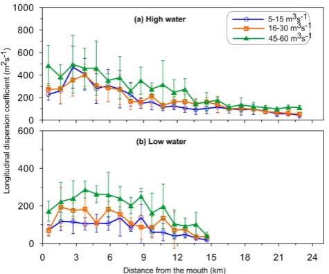
The relative abundance of salinity data in the SRE is used to estimate the distribution of the effective dispersionD(x), which varies with time and location. The longitudinal dispersion increases with increasing river discharge (45– 60 m3s−1) and decreases with diminishing river discharges (5–15 m3s−1). The range of dispersion coefficient values is rather broad for HWS (Fig. 4a). The values vary between 100 and 494 m2s−1, with a mean value of 261 m2s−1, at high tide for river discharge of 45–60 m3s−1. The mean longitudinal dispersions are 171 m2s−1 with a range of 44–470 m2s−1 for river discharges of 5–15 m3s−1, and 181 m2s−1 with a range of 53–400 m2s−1for river discharges of 16–30 m3s−1 at HWS. The spatially dependent structure has maximum mean values (>300 m2s−1) due to the reduced salinity gra-dient near the mouth. This reduced gragra-dient reflects a larger dispersion coefficient with higher standard deviation, and de-creases gradually upstream after the tidal excursion length at HWS.
[image:4.595.311.546.63.265.2]Table 1. Summary of the estimated longitudinal dispersion coefficient for different estuaries.
Source Estuary Longitudinal dispersion
coefficient (m2s−1)
West and Williams (1972) Ems estuary 50–300
Prandle (1981) A group of six estuaries 50–500
Van de Kreeke (1990) Volkerak estuary 150–325
Vallino and Hopkinson (1998) Parker River estuary 670 (near mouth)
de Swart et al. (1997) Ems estuary 200–1200
Lewis and Uncles (2003) Tees estuary 100
Lewis and Uncles (2003) Severn estuary 212
Austin (2004) Chesapeake Bay 200–1000, with a mean 650
Banas et al. (2004) Willapa bay 710 (near the mouth)
20 (upstream)
Fig. 4. Mean longitudinal dispersion coefficientDi (m2s−1) as a function of position along the Sumjin River Estuary for high water slack and low water slack conditions.
for a group of six estuaries. This range is consistent with that found at HWS in this study. However, de Swart et al. (1997) and Austin (2004) found a more wide range of dispersion coefficient. This inconsistency may be due to the variation in geometry and bathymetry of the estuaries. Ba-nas et al. (2004) also found a decreasing trend inDi(x)from
710 m2s−1near the mouth to 20 m2s−1upstream, in agree-ment with this study. Vallino and Hopkinson (1998) found a dispersion coefficient of 670 m2s−1near the mouth of Parker River estuary. These values correspond with the maximum dispersion coefficient during high tide of this study.
In contrast, the range of longitudinal dispersion coeffi-cient values is considerably smaller for LWS. These values range between 35 and 194 m2s−1, with a mean value of 110 m2s−1 for river discharge of 16–30 m3s−1 at low tide
(Fig. 4b). The mean value ofDi(x)is around 79 m2s−1with
a range of 18–138 m2s−1for river discharge of 5–15 m3s−1 and 184 m2s−1with a range of 41–286 m2s−1for river dis-charge of 45–60 m3s−1(Table 2). West and Williams (1972) found a range ofDi(x)values between 50 and 300 m2s−1in
Ems estuary, in agreement with this result. This also seems consistent with the result of Van de Kreeke (1990) who found a value between 150 and 325 m2s−1 in Volkerak estuary. Monismith (2010) gives a range of values forD(x), with typ-ical dispersion values of 100–300 m2s−1for many estuaries. Lewis and Uncles (2003) suggested a representative longi-tudinal dispersion value of 100 m2s−1 as a reasonable first choice for establishing a cross-sectionally averaged estuary model. Fischer et al. (1979) reported a typical dispersion value of 200 m2s−1for estuaries, particularly for tidal dis-persion. These average values of this study are consistent with those suggested by Fischer et al. (1979), Lewis and Un-cles (2003), and Monismith (2010).
The analysis of this study does not address the specific mechanisms responsible for this dispersion owing to a lack of velocity measurements. However, this quantitative knowl-edge of the spatially varying dispersive characteristics of the SRE can be useful for developing and testing hypotheses about various mixing mechanisms. This is the only example known to the authors of either temporal or spatial variabil-ity in dispersion estimates at high and low tide for the SRE. These data provide an important starting point for additional characterization of mixing processes in the SRE.
4.3 Effects of river discharge and potential energy anomaly on longitudinal dispersion
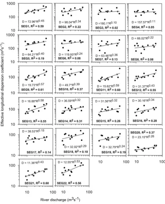
[image:5.595.50.288.267.465.2]Fig. 5. Effective longitudinal dispersion coefficient (D) estimated at high water slack versus river discharge (R) at various positions along the Sumjin River Estuary.
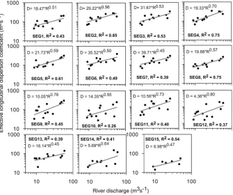
a function of the square root of the river discharge (Eqs. 1.2 and 5.70; Savenije, 2005). The dispersion varies approxi-mately with the root of the freshwater discharge in segments 1, 9, 11, 12, 13, 21 and 22 at HWS (Fig. 5). Some loca-tions do not show this functional relaloca-tionship between river discharge and longitudinal dispersion coefficient at high tide. This is because mixing in estuaries is determined in part by the bathymetry, and no combination of purely external inputs completely describes the process (Fischer, 1976). Moreover, Chatwin and Allen (1985) reported that the transport of salt at a given point in space may conveniently be considered to result from turbulent mean advection processes and turbu-lent diffusion processes. At LWS, the dispersion varies with the root of the freshwater discharge mostly in all segments except in 4, 9, 11, 12 and 13 (Fig. 6). As the tidal effect
is minimal at LWS compared to that at HWS, and river dis-charge induces seaward advection at LWS, a more functional relationship between river discharge and longitudinal disper-sion coefficient might be found at LWS than at HWS. Ward and Fischer (1971) noted that althoughD(x,t )is a function of discharge at any given location for a range of dispersion values, the variability inD(x,t )atxcould be due to the ex-treme complexity of estuarine systems including great vari-ation in geometry and bathymetry as well as inappropriate application of the steady-state assumption for some salinity distributions because freshwater discharge varies over sev-eral orders of magnitude during the course of a year.
Fig. 6. Effective longitudinal dispersion coefficient (D) estimated at low water slack versus river discharge (R) at various positions along the Sumjin River Estuary.
Table 2. Longitudinal dispersion coefficients of the SRE for different river discharges.
Tide River discharge Minimum Average Maximum (m3s−1) (m2s−1, upstream) (m2s−1) (m2s−1, near mouth)
HWS
5–15 44 171 470 16–30 53 181 400 45–60 100 261 494
LWS
5–15 18 79 138 16–30 35 110 194 45–60 41 184 286
The tidal height data were collected from the Gwangyang tidal gauge station near the SRE’s mouth. These data were used to examine the effects of tidal heights on the longitu-dinal dispersion coefficient because of a lack of observed tidal height data along the SRE. This may be one cause of an insignificant correlation between tidal height and longitu-dinal dispersion coefficient. This is attributed to turbulence generated by strong tidal currents, which effectively reduce the dispersing action of velocity shears (Linden and Simp-son, 1988). Without corresponding velocity data (the obser-vations lack velocity measurements), it is impossible to judge the relative contribution of shear flow dispersion by tidal cur-rents. However, the fact that the dispersion increases with river discharge is consistent with previous studies.
The spatial variation in the potential energy anomaly at low and high tides along the SRE is shown in Fig. 7. The potential energy anomaly (φ) is the amount of work neces-sary to completely mix the water column (Jm−3) and can be calculated usingφ= 1
H
0
R
−H
gz(ρ−ρ)dz, whereρ is the ver-tical density profile over a water column of depthH, zis the vertical coordinate andgis the gravitational acceleration (9.8 m s−2). The potential energy anomaly increases with in-creasing river discharges. As a result, the longitudinal disper-sion increases with increasing potential energy on the water column. The potential energy anomaly at HWS (Fig. 7a) is
[image:7.595.49.286.437.518.2]Fig. 7. Spatial variation in the potential energy anomaly at low
and high tides along the Sumjin River Estuary under different river discharges.
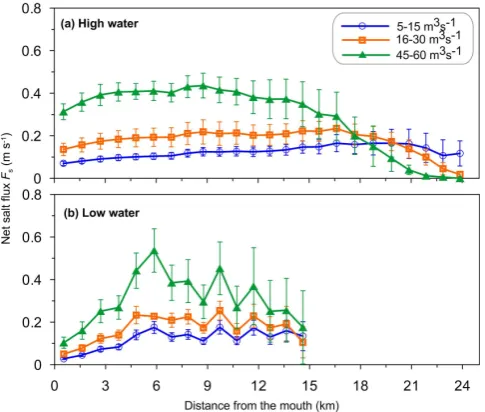
Fig. 8. Response of dispersive salt fluxFs(m s−1) to salinity
gradi-ent (km−1) at low and high waters along the Sumjin River Estuary under different river discharges.
scale observed in the SRE (Shaha and Cho, 2009). Banas et al. (2004) also found the maximumD(x)value near the mouth. In contrast,φincreased to more than 11 Jm−3 land-ward from the tidal excursion length of 6 km, and the value ofD(x)decreased upstream.
4.4 Link between salt fluxes and salinity gradient
The spatially varying horizontal dispersion coefficient is in-versely related to the salinity gradient; whereas the salt fluxes are proportional to the salinity gradient (Fig. 8). The low salt fluxes are associated with low salinity gradients and a low potential energy anomaly, whereas high salt fluxes are asso-ciated with high salinity gradients and a high potential energy anomaly. The net salt fluxes increases with increasing river discharges and decreases with decreasing river discharges at HWS and LWS (Fig. 8a–b).
As the cross-sectional area increases exponentially at the seaward end of the SRE (Shaha and Cho, 2011), the displacement of the salinity distribution for a particular iso-haline decreases at the seaward end of the SRE. Therefore, the seaward advective transport of salt per unit area decreases to the mouth of the SRE from the upstream end at LWS be-cause of maintaining mass balance. This result is consistent with that of Lewis and Uncles (2003). They reported that the rate of salt transport per unit area at the seaward end of a coastal plain estuary may be quite small because of the rela-tively large cross-sectional area, which leads to low residual currents.
On the other hand, the salt fluxes increase in the central regimes owing to the increasing salinity gradient. The sea-ward shifts of the salinity distribution in the central and inner regimes are much more sensitive at LWS than at HWS during high river discharge period because of mass balance between the regions of greater cross-sectional area (near the mouth) and shorter cross-sectional area (upstream). As a result the standard deviation of net salt fluxes is higher in the central regimes at LWS than at HWS.
5 Conclusions
[image:8.595.47.290.334.540.2]river discharges at both HWS and LWS in many locations along the SRE which are consistent with the theory.
The salinity gradient decreases at the seaward end of the SRE and increases upstream by maintaining mass balance between greater cross-section area near the mouth and up-stream locations. The dispersive flux of salt is particularly sensitive near the maximum salinity gradient in the central regimes at LWS because of the increasing displacement of isohalines. The salt flux increases with the salinity gradient and potential energy anomaly at both LWS and HWS.
These basic estimates of effective longitudinal dispersion and information about their spatial and temporal variability will provide an essential test for numerical models of this es-tuarine circulation. A better understanding of the principal hydraulic parameters controlling mixing such as the disper-sion coefficient is therefore the prime requirement for an ef-fective numerical simulation of estuarine circulation. Longi-tudinal velocity measurements using ADCP and experiment of 3-D numerical model will be performed to verify and re-fine the dispersion coefficients determined from salinity dis-tribution in the next study.
Acknowledgements. This research was supported by the NAP
program of the Korea Ocean Research Development Institute and the project titled on “Long-term change of structure and function in marine ecosystems of Korea” funded by the Ministry of Land,
Transport and Maritime Affairs, Korea. The authors thank the
members of the Marine Environment Prediction Laboratory for their enthusiastic supports during data collection.
Edited by: H. H. G. Savenije
References
Austin, J. A.: Estimation of effective longitudinal dispersion in the Chesapeake Bay, Estuar. Coast. Shelf S., 60, 359–368, 2004. Bae, D. H., Jung, I. W., and Chang, H.: Long-term trend of
precip-itation and runoff in Korean river basins, Hydrol. Process., 22, 2644–2656, 2008.
Banas, N. S., Hickey, B. M., MacCready, P., and Newton, J. A.: Dy-namics of Willapa Bay, Washington, a highly unsteady partially mixed estuary, J. Phys. Ocean., 34, 2413–2427, 2004.
Burchard, H. and Hofmeister, R.: A dynamic equation for the po-tential energy anomaly for analysing mixing and stratification in estuaries and coastal seas, Estuar. Coast. Shelf S., 77, 679–687, 2008.
Caplow, T., Schlosser, P., Ho, D. T., and Santella, N.: Transport dy-namics in a sheltered estuary and connecting tidal straits: SF6
tracer study in New York Harbor, Environ. Sci. Technol., 37, 5116–5126, 2003.
Chatwin, P. C. and Allen, C. M.: Mathematical models of dispersion in rivers and estuaries, Ann. Rev. Fluid. Mech., 17, 119–149, 1985.
de Swart, H. E., De Jonge, V. N., and Vosbeek, M.: Application of the tidal random walk model to calculate water dispersion coef-ficients in the Ems estuary, Estuar. Coast. Shelf S., 45, 123–133, 1997.
Dyer, K. R.: Estuaries, A Physical Introduction, 2nd Edn., John Wiley, London, 195 pp., 1997.
Eaton, T. T.: Analytical estimates of hydraulic parameters for an ur-banized estuary – Flushing Bay, J. Hydrol., 347, 188–196, 2007. Fischer, H. B.: Mixing and dispersion in estuaries, Ann. Rev. Fluid
Mech., 8, 107–133, 1976.
Fischer, H. B., List, E. J., Koh, R. C. Y., Imberger, J., and Brooks, N. H.: Mixing in Inland and Coastal Waters, 1st Edn, Academic Press, New York, 483 pp., 1979.
Garcia-Barcina, J. M., Gonzalez-Oreja, J. A., and De la Sota, A.: Assessing the improvement of the Bilbao estuary water quality in response to pollution abatement measures, Water Res. 40, 951– 960, 2006.
Garvine, R., McCarthy, R., and Wong, K.-C.: The axial salinity dis-tribution in the Delaware estuary and its weak response to river discharge, Estuar. Coast. Shelf S., 35, 157–165, 1992.
Gay, P. and O’Donnell, J.: Comparison of the salinity structure of the Chesapeake bay, the Delaware bay and long Island sound us-ing a linearly tapered advection-dispersion model, Estuar. Coast., 32, 68–87, doi:10.1007/s12237-008-9101-4, 2009.
Geyer, W. and Signell, R.: A reassessment of the role of tidal dis-persion in estuaries and bays, Estuar. Coast., 15, 97–108, 1992. Guymer, I. and West, J. R.: The determination of estuarine
diffu-sion coefficients using a fluorimetric dye tracing technique, J. Hydraul. Eng., 118, 718–734, 1992.
Ho, D. T., Schlosser, P., and Caplow, T.: Determination of longitu-dinal dispersion coefficient and net advection in the tidal Hudson River with a large-scale, high resolution SF6tracer release ex-periment, Environ. Sci. Technol., 36, 3234–3241, 2002. Ji, Z. G.: Hydrodynamics and Water Quality: Modeling Rivers,
Lakes and Estuaries, 1st Edn., John Wiley, New Jersey, USA, 676 pp., 2008.
Lewis, R. E. and Uncles, R. J.: Factors affecting longitudinal disper-sion in estuaries of different scale, Ocean Dynam., 53, 197–207, 2003.
Linden, P. F. and Simpson, J. E.: Modulated mixing and frontogene-sis in shallow seas and estuaries, Cont. Shelf Res., 8, 1107–1127, 1988.
MacCready, P.: Estuarine adjustment to changes in river flow and tidal mixing, J. Phys. Oceanogr., 29, 708–726, 1999.
MacCready, P. and Geyer, W. R.: Advances in estuarine physics, Annu. Rev. Mar. Sci., 2, 35–58, 2010.
Monismith, S. G.: Mixing in estuaries, in: Contemporary Issues in Estuarine Physics, edited by: Valle-Levinson, A, Cambridge University Press, Cambridge, 145–185, 2010.
Monismith, S. G., Kimmerer, W., Stacey, M. T., and Burau, J. R.: Structure and flow-induced variability of the subtidal salinity field in Northern San Francisco Bay, J. Phys. Ocean., 32, 3003– 3019, 2002.
Officer, C. B.: Physical Oceanography of Estuaries (and Associated Coastal Waters), John Wiley, New York, USA, 465 pp., 1976. Paulson, R. W.: Variation of the longitudinal dispersion coefficient
in the Delaware River Estuary as a function of freshwater inflow, Water Resour. Res., 6, 516–526, 1970.
Prandle, D.: Salinity intrusion in estuaries, J. Phys. Oceanogr., 11, 1311–1324, 1981.
Savenije, H. H. G.: A one-dimensional model for salinity intrusion in alluvial estuaries, J. Hydrol., 85, 87–109, 1986.
water slack and mean tide on spreadsheet, J. Hydrol., 107, 9–18, 1989.
Savenije, H. H. G.: Salinity and Tides in Alluvial Estuaries, 1st Edn., Elsevier, Amsterdam, 197 pp., 2005.
Shaha, D. C. and Cho, Y.-K.: Comparison of empirical models with intensively observed data for prediction of salt intrusion in the Sumjin River estuary, Korea, Hydrol. Earth Syst. Sci., 13, 923– 933, doi:10.5194/hess-13-923-2009, 2009.
Shaha, D. C. and Cho, Y.-K.: Determination of spatially varying Van der Burgh’s coefficient from estuarine parameter to describe salt transport in an estuary, Hydrol. Earth Syst. Sci., 15, 1369– 1377, doi:10.5194/hess-15-1369-2011, 2011.
Shaha, D. C., Cho, Y.-K., Seo, G.-H., Kim, C.-S., and Jung, K. T.: Using flushing rate to investigate spring-neap and spatial varia-tions of gravitational circulation and tidal exchanges in an estu-ary, Hydrol. Earth Syst. Sci., 14, 1465–1476, doi:10.5194/hess-14-1465-2010, 2010.
Vallino, J. J. and Hopkinson, Jr. C. S.: Estimation of dispersion and characteristic mixing times in Plum Island Sound Estuary, Estuar. Coast. Shelf S., 46, 333–350, 1998.
Van de Kreeke, J.: Longitudinal dispersion in the Volkerak Estuary, in: Cheng RT, Residual currents and long-term transport, Lecture notes on coastal and estuarine studies, Springer, Berlin Heidel-berg New York, 38, 151–164, 1990.
Ward, P. R. B. and Fischer, H. B.: Some limitations on use of the one-dimensional dispersion equation, with comments on two pa-pers by: R. W. Paulson, Water Resour. Res., 7, 215–220, 1971. West, J. R. and Williams, J. R. A.: An evaluation of mixing in the