Uncertainty analysis in model parameters regionalization: a case study involving the SWAT model in Mediterranean catchments (Southern France)

www.hydrol-earth-syst-sci.net/18/2393/2014/ doi:10.5194/hess-18-2393-2014

© Author(s) 2014. CC Attribution 3.0 License.

Uncertainty analysis in model parameters regionalization: a case

study involving the SWAT model in Mediterranean catchments

(Southern France)

H. Sellami1, I. La Jeunesse2,3, S. Benabdallah4, N. Baghdadi5, and M. Vanclooster1

1_{Earth and Life Institute, Université catholique de Louvain, Croix du Sud 2, Box 2, 1348 Louvain-la-Neuve, Belgium} 2_{UMR 7324 CITERES, Université de Tours, 33 allée Ferdinand de Lesseps BP 60449 – 37204 Tours cedex 3, France} 3_{LETG-Angers LEESA, UMR 6554 CNRS, Université d’Angers, Faculté des Sciences, 2 Bd Lavoisier,}

49045 Angers Cedex 1, France

4_{Centre de Recherches et des Technologies des Eaux, Technopole Borj Cedria, BP 273, Soliman 8020, Tunisia} 5_{IRSTEA, UMR TETIS, 500 rue François Breton, 34093 Montpellier CEDEX 5, France}

Correspondence to: H. Sellami ([email protected])

Received: 4 February 2013 – Published in Hydrol. Earth Syst. Sci. Discuss.: 18 April 2013 Revised: 29 April 2014 – Accepted: 22 May 2014 – Published: 26 June 2014

Abstract. In this study a method for propagating the hy-drological model uncertainty in discharge predictions of un-gauged Mediterranean catchments using a model parameter regionalization approach is presented. The method is devel-oped and tested for the Thau catchment located in Southern France using the SWAT hydrological model. Regionaliza-tion of model parameters, based on physical similarity mea-sured between gauged and ungauged catchment attributes, is a popular methodology for discharge prediction in ungauged basins, but it is often confronted with an arbitrary criterion for selecting the “behavioral” model parameter sets (Mps) at the gauged catchment. A more objective method is provided in this paper where the transferrable Mps are selected based on the similarity between the donor and the receptor catch-ments. In addition, the method allows propagating the mod-eling uncertainty while transferring the Mps to the ungauged catchments. Results indicate that physically similar catch-ments located within the same geographic and climatic re-gion may exhibit similar hydrological behavior and can also be affected by similar model prediction uncertainty. Further-more, the results suggest that model prediction uncertainty at the ungauged catchment increases as the dissimilarity be-tween the donor and the receptor catchments increases. The methodology presented in this paper can be replicated and used in regionalization of any hydrological model parame-ters for estimating streamflow at ungauged catchment.

1 Introduction

al., 2005; McIntyre et al., 2005). On the other hand, region-alization based on a similarity approach consists of trans-ferring the information from donor catchment(s) to recep-tor catchment(s). It starts by identifying one or more donor catchments, which are usually gauged catchments that are most likely to be hydrologically similar to one or more re-ceptor catchments. Then, the relevant information (Mps or streamflow records) is transferred from donor to receptor catchments. Typically, Mps transferred from donor to recep-tor catchment(s) rely on physical similarity measures. In this case, the same CAs as used in the statistical technique can be adopted to identify similar catchments. Alternatively, use can be made of spatial proximity measures (e.g., the dis-tance between the centroids of the catchments). The simi-larity regionalization approach is based on the assumption that similar catchments behave hydrologically similarly. So, the definition of the similarity measure, certainly subjective, will condition the success of the selected regionalization ap-proach (Heuvelmans et al., 2006).

Several studies have focused on the transfer of Mps based on similarity approach for predicting streamflow records at ungauged catchments (Merz and Blöschl, 2004; McIntyre et al., 2005; Parajka et al., 2005; Bàrdossy, 2007; Oudin et al., 2008). For instance, McIntyre et al. (2005) found that Mps transfer outperformed as compared to the statistical regres-sion approach using a five-parameter verregres-sion of the proba-bility distribution model (Moore, 1985) applied to 127 UK catchments. Similar conclusions were drawn by Oudin et al. (2008) using two conceptual rainfall–runoff models on 913 French catchments; the GR4J (modèle du Génie Rural à 4 paramètres Journalier) developed by Perrin et al. (2003) and the TOPMO model, which is a six-parameter version of the TOPMODEL (Beven, 1997). Parajka et al. (2005) used four groups of regionalization approaches. The first group is based on spatial averaging of calibrated model parameters, the second is based on spatial proximity (spatial distance) tween the catchments, the third uses multiple regression be-tween catchment attributes and model parameters and the last group is based on similarity between catchment attributes. They have found that regionalization methods based on spa-tial proximity and catchment attributes similarity performed better than multiple regression and spatial averaging meth-ods. However, other studies have reported that even nearby catchments can be hydrologically different (Ouarda et al., 2001; Shu and Burn, 2003; McIntyre et al., 2005; Beven, 2000).

The similarity approach for the regionalization of Mps in ungauged catchments implies the “good” performance of the calibrated hydrological model at the donor catchment. Then, Mps that lead to “good” or “behavioral” model sim-ulations are selected and transferred to the ungauged catch-ment. However, it is argued that hydrological model predic-tions, even in well-gauged catchments, are subject to inher-ent uncertainty that stems from differinher-ent uncertainty sources (e.g., inputs, parameter uncertainty, model structure, and

ob-served data). Because of all these uncertainty sources, it is expected and argued that model calibration will lead to non-unique sets of parameters (Beven and Binley, 1992). There-fore, it becomes difficult to associate the calibrated parame-ters with the physical characteristics of the catchment.

While model parameter uncertainty at well-gauged catch-ments has received considerable attention during the past two decades (Beven and Binley, 1992; Duan et al., 1992; Ab-baspour et al., 1997; Muleta and Nicklow, 2005; Vrugt et al., 2008; Yang et al., 2008; Zhang et al., 2009; Shen et al., 2012), little attention has been given to the uncertainty resulting from Mps regionalization at ungauged sites (Wagener and Wheater, 2006). Furthermore, with additional uncertainty re-lated to the regionalization procedure that stems from the ar-bitrary choices of the CAs, the similarity measure, the selec-tion of the candidate parameter sets to be transferred can have a significant effect on the model prediction uncertainty in the ungauged catchments. Addressing all these sources of uncer-tainty and understanding the way they can affect the model prediction in the ungauged catchment is a challenging task (Sivapalan et al., 2003; Wagener et al., 2004).

This paper aims to contribute to this challenge by ad-dressing the following question: how can Mps uncertainty of donor catchments be propagated through regionalization schemes based on the similarity approach, and how does it affect the prediction uncertainty in ungauged catchments? Specific questions are as follows: (1) is the selected hydro-logical model suitable for reproducing the hydrology in the ungauged catchment? (2) How does parameter uncertainty affect model prediction uncertainty in the ungauged catch-ment through the regionalization scheme?

In an attempt to answer to these research questions, the pa-per is organized in three main sections. In the first section the study site, the data available, the modeling approach and the regionalization procedure are described. The second section describes and discusses the results of the modeling and the regionalization approach. The final section reports the main outcomes of the paper as a summary of conclusions.

2 Study site description and available data 2.1 Study site description

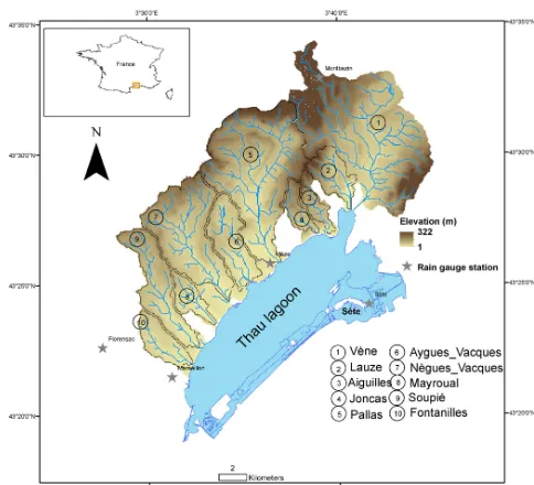
Figure 1. Location, topography, rain gauge stations and

subcatch-ment boundaries of the Thau Basin.

Thau catchment area is composed of Jurassic limestone over-laid by Miocene marls in its central part, corresponding to 60 % of the Vène watershed surface. This Jurassic limestone is characterized by the presence of a large karstic aquifer whose limits extend the topographic limit of the catchment and strongly influences the hydrological regime of the Vène catchment (Plus et al., 2006; Gallart et al., 2008; Perrin and Tournoud, 2009; Sellami et al., 2013). Soils in this part of the Thau catchment are mainly sandy-loam and silty-loam soils with porosity ranging from 35 to 50 % at 1 m depth of the soil profile. The western part of the Thau catchment is composed of the Eocene marls overlaid mainly by the Miocene marls. This region covers the central part of the Pal-las, Aygues_Vacques, Nègues_Vacques, Mayroual, Soupié and Fontanilles catchments with silty-clayey-loam and loam-textured soils so that runoff generation process are expected to be different from the eastern part.

2.2 Available data

The climate is a typical Mediterranean regime characterized by a large seasonal variability of rainfall in time and space with an annual average value of 600 mm. Precipitation oc-curs as short intense storms mainly during autumn and spring (from September to January) and separated by a long dry period (from February to August). The hottest months are July and August where the maximum temperature can ex-ceed 35◦C and the coldest months are December and January where daily minimum temperature can reach−5◦C.

Data from resources such as a digital elevation model (50 m grid, provided by the French National Geographic In-stitute), a soil map (50 m resolution, provided by the INRA

Figure 2. Land use distribution in the Vène and in the Pallas

water-sheds for 1996 and 2010.

Montpellier) and land use maps (50 m resolution) for 1996 (La Jeunesse et al., 2002) and 2010 are available for each catchment. Daily precipitation data (from 1990 to 1999) are provided by five rain gauge stations located within the study area (Fig. 1) but only the Sète rain gauge (French national meteorological station of Météo France) has daily precipi-tation data from 1990 to 2009. Daily temperatures are pro-vided from the meteorological station of Sète. Wind speed, air relative humidity and solar radiation daily data are pro-vided from the meteorological station of Fréjorgues airport located 20 km in the northeastern of the Thau catchment.

In the Thau Basin about 2 years (1994–1996) of stream-flow records are available for the Vène and the Pallas catch-ments, while for the other rivers, streamflow records are ei-ther missing or have missing values and are not long enough to allow direct model calibration. The lengths of the avail-able streamflow records, as well as their corresponding time periods, for each catchment are summarized in Table 1. Such cases of poorly gauged catchments is very common in semi-arid and Mediterranean areas and, when coupled with dis-continuities in flow regime of ephemeral rivers, makes the modeling of the discharge challenging.

Table 1. Discharge and precipitation data available for each catchment.

Catchment Discharge Observations Precipitation name time period length (days) time period

Vène 1994–1996 667 1990–2010

Pallas 1994–1996 208 1990–2010

Lauze NA NA 1990–1999

Aiguilles NA NA 1990–1999

Joncas 2007–2009 81 1990–1999

Aygues_Vacques 2007–2009 85 1990–1999

Nègues_Vacques NA NA 1990–1999

Mayroual NA NA 1990–1999

Soupié 2007–2009 536 1990–1999

Fontanilles 2007–2009 540 1990–1999

Note: NA means not available.

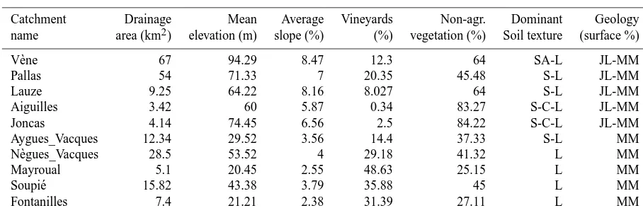
Table 2. Description of the catchments attributes.

Catchment Drainage Mean Average Vineyards Non-agr. Dominant Geology

name area (km2) elevation (m) slope (%) (%) vegetation (%) Soil texture (surface %)

Vène 67 94.29 8.47 12.3 64 SA-L JL-MM

Pallas 54 71.33 7 20.35 45.48 S-L JL-MM

Lauze 9.25 64.22 8.16 8.027 64 S-L JL-MM

Aiguilles 3.42 60 5.87 0.34 83.27 S-C-L JL-MM

Joncas 4.14 74.45 6.56 2.5 84.22 S-C-L JL-MM

Aygues_Vacques 12.34 29.52 3.56 14.4 37.33 S-L MM

Nègues_Vacques 28.5 53.52 4 29.18 41.32 L MM

Mayroual 5.1 20.45 2.55 48.63 25.15 L MM

Soupié 15.82 43.38 3.79 35.88 45 L MM

Fontanilles 7.4 21.21 2.38 31.39 27.11 L MM

Note: Soil code: SA-L: sandy loam, S-L: silty loam, S-C-L: silty clayey loam and L: loam. Geology code: JL, Jurassic Limestone; MM, Miocene Marls.

model parameter regionalization approach results is, how-ever, not within the objectives of this paper.

As the Pallas and the Vène catchments have been subject to many previous studies (Aquilina et al., 2002; La Jeunesse et al., 2002; Plus et al., 2006; Chahinian et al., 2011; Sellami et al., 2013), more detailed data are available for these sub-catchments. Therefore, the Vène and the Pallas catchments are considered as gauged catchments, while all other small catchments are considered ungauged.

3 Description of the hydrological model

The Soil and Water Assessment Tool (SWAT) (Arnold et al., 1998) is a continuous-time and physically based hydrologi-cal model. SWAT is developed to predict the impact of land management practices on water, sediment and agricultural chemical yields in large complex catchments with different soil, land use and management conditions over long periods of time (Eckhardt et al., 2005). The hydrological model op-erates by dividing the watershed into subbasins. Each sub-basin is further discretized into a series of hydrologic

re-sponse units (HRUs), which are unique soil–land use com-binations. Soil water content, surface runoff, nutrient cycles, sediment yield, crop growth and management practices are simulated for each HRU and then aggregated for the subbasin by a weighted average. The hydrological balance is calcu-lated based on the following equation:

∂SW

∂t =Pday−Qsurf−Ea−Wseep−Qgw (1)

where SW is the soil water content (mm), Pday is pre-cipitation rate (mm day−1), Qsurf is the surface runoff rate (mm day−1),Eais evapotranspiration rate (mm day−1), Wseep is the water percolation rate from the soil pro-file (mm day−1_{), and Q}

gw is the groundwater flow rate (mm day−1_).

routed through the river channel using the variable storage or Muskingum method. The watershed concentration time is estimated using Manning’s kinematic equation, considering both overland and channel flow.

The soil profile is subdivided into multiple layers that sup-port soil water processes including infiltration, evaporation, plant uptake, lateral flow, and percolation to lower layers. The soil percolation component of SWAT uses a water stor-age capacity technique to predict flow through each soil layer in the root zone. Downward flow occurs when field capac-ity of a soil layer is exceeded and the layer below is not saturated. Percolation from the bottom of the soil profile recharges the shallow aquifer. The amount of water entering the shallow aquifer is a function of the total water volume exiting the soil profile and an exponential decay function to account for the recharge time delay. The latter depends on the overlying geologic formations. If the depth of the shallow aquifer increases above the user-defined threshold value, it is assumed that groundwater discharge occurs and contributes to the reach. Upward flow movement to the overlaying unsat-urated soil layers is simulated by routing water in the shallow aquifer storage component to the soil by capillary pressure or by direct absorption by the plant roots. This water removal process is termed “revap”.

The model computes evaporation from soils and plants separately. Potential evapotranspiration can be modeled with three options available in SWAT, that is, the Penman– Monteith, Priestley–Taylor and Hargreaves methods (Neitsch et al., 2005), depending on data availability. Potential soil water evaporation is estimated as a function of potential ET and leaf area index. Actual soil evaporation is estimated by using exponential functions of soil depth and water content. Plant water evaporation is simulated as a linear function of potential ET, leaf area index, and root depth, and can be lim-ited by soil water content. More detailed descriptions of the SWAT model can be found in Neitsch et al. (2005).

The SWAT simulations are conducted on the gauged catch-ments from 1990 to 1996 on a daily time step. However, due to the complex nature of the flow processes and the presence of the karstic system in the catchment, a model warm-up pe-riod of 4 years (1990–1993) is considered to be sufficient to minimize the effects of the initial state of the SWAT vari-ables on the river flow prediction (Sellami et al., 2013). The modified SCS curve number method is chosen for surface runoff volume computing. The variable storage coefficient method is selected for the flow routing through the channel and potential evapotranspiration is estimated by the Penman– Monteith method. The daily stream flow data from 2 Au-gust 1994 to 1 July 1996 and from 25 November 1995 to 14 June 1996 for the Vène and the Pallas catchments, respec-tively, are used to assess the model prediction performances.

4 Modeling approach 4.1 Sensitivity analysis (SA)

A way to deal with high-dimensional hydrological models, such as SWAT, is to conduct SA to select only the sensitive model parameters that are assumed to represent the real sys-tem behavior. In the current case study, a SA is conducted using the built-in SWAT SA tool that uses the Latin Hy-percube One-factor-At-a-Time (LH-OAT) (van Griensven et al., 2006) method. In the LH-OAT technique only one input parameter is modified between two successive model runs. Therefore, the change in model output can then be attributed to such parameter modification. In this study, the parameter that induces the highest model output change is ranked first and the less sensitive parameter is given a rank equal to zero. A complete detailed explanation of this SA technique can be found in van Griensven et al. (2006).

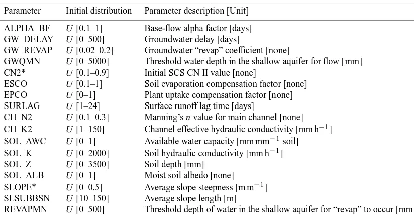
Table 3. Initial range, sensitivity analysis results and description of the selected SWAT model parameters.

Parameter Initial distribution Parameter description [Unit]

ALPHA_BF U[0.1–1] Base-flow alpha factor [days] GW_DELAY U[0–500] Groundwater delay [days]

GW_REVAP U[0.02–0.2] Groundwater “revap” coefficient [none]

GWQMN U[0–5000] Threshold water depth in the shallow aquifer for flow [mm] CN2* U[0.1–0.9] Initial SCS CN II value [none]

ESCO U[0.1–1] Soil evaporation compensation factor [none] EPCO U[0–1] Plant uptake compensation factor [none] SURLAG U[1–24] Surface runoff lag time [days]

CH_N2 U[0.1–0.3] Manning’snvalue for main channel [none] CH_K2 U[1–150] Channel effective hydraulic conductivity [mm h−1] SOL_AWC U[0–1] Available water capacity [mm mm−1soil] SOL_K U[0–2000] Soil hydraulic conductivity [mm h−1]

SOL_Z U[0–3500] Soil depth [mm]

SOL_ALB U[0–1] Moist soil albedo [none] SLOPE* U[0–0.5] Average slope steepness [m m−1] SLSUBBSN U[10–150] Average slope length [m]

REVAPMN U[0–500] Threshold depth of water in the shallow aquifer for “revap” to occur [mm]

Note:Umeans uniform distribution. * Means fraction of variation by which the initial value of the parameter is changed. The rank zero is attributed to parameter that is not considered as sensitive.

water movement between the root zone and the shallow aquifer; and SURLAG, which controls the fraction of the to-tal water that is allowed to enter the stream on any specific day.

It is argued that in order to provide better identified mod-els and to ensure high regionalization potential, the struc-ture of the selected hydrological model should be reduced to only components that describe the key process of the system. Therefore, it is suggested that the number of required model parameters should not be more than half a dozen (Wagener et al., 2001). However, the approach to retain only the neces-sary model structure components (parsimonious model) do not necessary guarantee that all the hydrological processes of the watershed are identified and represented, especially in complex hydrological systems. However, from the results of the SA and the physical meaning of the selected sensitive parameters it is obviously difficult to select less than 10 pa-rameters in the current study. In addition, it is well known that the hydrological processes are complex in the study area due to the presence of the karstic aquifer in the Vène wa-tershed (Plus et al., 2006; Gallart et al., 2008; Perrin and Tournoud, 2009; Chahinian et al., 2011). Hence, selecting the 10 sensitive parameters described above ensures that the model does not omit 1 or more hydrological processes impor-tant for this particular case study. Furthermore, other studies dealing with the SWAT model have identified more or less 10 sensitive parameters that are assumed to describe appro-priately the hydrological process of the real system. For ex-ample, Heuvelmans et al. (2004) have identified seven sensi-tive SWAT model parameters related to flow generation to be regionalized in northern Belgium. Gitau and Chaubey (2010)

have selected 16 SWAT parameters for flow prediction in un-gauged catchments. Chahinian et al. (2011) have calibrated 14 SWAT model parameters for modeling flow and nutrient emission processes. They found that 12 sensitive parameters are directly and indirectly related to flow simulation.

4.2 Uncertainty analysis (UA)

which is also used in this study. Other subjective choices are considered within the implementation of the GLUE frame-work in this study. The prior distributions of the selected pa-rameters are assumed to follow a uniform distribution over their respective range (Table 3). This initial distribution is chosen since the real distribution of the parameter is un-known. The ranges of the parameters are chosen based on the SWAT manual (Neitsch et al., 2005) and previous ap-plications of the technique with the SWAT model (Yang et al., 2008; Shen et al., 2012). To sample the prior parameter distribution, a simple random sampling is implemented. The number of sampling sets is set to 10 000. Such a number of simulations was identified as sufficient for assessing uncer-tainty of about 10 sensitive SWAT model parameters (Yang et al., 2008; Gong et al., 2011). Moreover, it was mentioned by Yang et al. (2008) that no significant change was observed in the GLUE results between 10 000 and 20 000 model runs. So the selected number of 10 000 simulations is considered reasonably sufficient for this study. The likelihood function selected is the Nash and Sutcliffe (1970) efficiency coeffi-cient (NS) since it is widely used as a likelihood measure in GLUE in the literature (Beven and Freer, 2001; Arabi et al., 2007; Shen et al., 2012).

NS=1− n

P

i=1

(Pi−Oi)2

n

P

i=1

Oi−O 2,

(2)

where Oi is the observed value,O mean observed values

andPi is the predicted value. The range of NS lies between

1 (perfect fit) and−∞.

The cutoff threshold selected to separate “behavioral” from “non-behavioral” parameter sets is another subjective choice within the GLUE method. Frequently, when the like-lihood value is greater than zero, the corresponding simula-tions are considered “behavioral” (Freni and Mannina, 2010; Gong et al., 2011). In this study, model simulations with negative NS values are considered unacceptable and, there-fore, the corresponding parameter sets are discarded from further analysis. The selection of the threshold value is an en-tirely arbitrary choice that affects the prediction uncertainty (Montanari, 2005; Mantovan and Todini, 2006) and proba-bly is the most important concern for the GLUE method. A small cutoff threshold will lead to larger “behavioral” sim-ulations and larger uncertainty bands, while larger thresh-old value will decrease the numbers of “behavioral” mod-els and will reduce the uncertainty interval width (Xiong and O’Connor, 2008; Blasone et al., 2008; Viola et al., 2009). As the GLUE method is dependent on all these subjective de-cisions that influence the final uncertainty prediction, it has been deeply criticized and its several drawbacks have been well pointed out and discussed in the literature (Montanari, 2005; Mantovan and Todini, 2006).

4.3 The regionalization schemes

The adopted regionalization method for this study is the transfer of Mps from donor to receptor catchment based on the similarity between their physical attributes (topography, geology, soils, drainage area, etc.). The physical similarity approach is based on the assumption that catchment phys-iographic characteristics predetermine the hydrological be-havior. Therefore, the selection of relevant CAs is crucial for the success of the regionalization procedure. The catch-ments attributes (CAs) selected and used to define similarity are related to topography, land cover, drainage area, soil and geology features (Table 2). They are derived from the avail-able data such as land use maps, soil maps, digital elevation model and geology maps. These CAs are generally consid-ered as the main drivers of the hydrological process in the literature (Merz and Blöschl, 2004; Heuvelmans et al., 2006; Wagener et al., 2007; Bastola et al., 2008) and are the most common ones used to define similarity between catchments in model parameter regionalization schemes. For instance, Heuvelmans et al. (2006) have considered catchment area, average slope, dominant land use and soil texture classes as the most appropriate catchment descriptors in model parame-ters regionalization in Flemish part of the Scheldt River basin (Belgium). Besides these CAs, other authors have used flow indices or characteristics using flow duration curve (FDC) (Masih et al., 2010), indices of hydrological responses (Ya-dav et al., 2007) or hydro-meteorological long-term data (Bastola et al., 2008) as relevant catchment descriptors. How-ever, the selection of the appropriate CAs also depends on the physical meaning of the selected model parameters, on the objective of the regionalization procedure and on the knowl-edge about the key hydrological processes occurring within the catchment. For example, when the objective of the re-gionalization procedure is to estimate the flow in ungauged catchments, as in our case, the use of flow characteristics or indices as input is useless. Model parameters, especially those of physically based models such as SWAT, are assumed to be closely related to CAs and, thus, to represent the func-tional behavior of the catchment response. For instance, in the SWAT model, the curve number parameter (CN2) de-pends on the soil and land use characteristics of the catch-ment, which are considered among the relevant catchment descriptors. Knowledge about the key processes in the sys-tem can also assist the selection of the relevant CAs. As an example, the geology is considered as a relevant catchment descriptor in our case study since it is known that the Juras-sic limestone aquifer in the eastern part of the Thau catch-ment strongly influences the hydrological regime of the Vène catchment (Sellami et al., 2013).

the GIS tools based on a simplified geological map of the Thau catchment. Other geomorphologic and topographic de-scriptors (mean elevation, mean slope, drainage area) are also calculated using GIS tools and are reported in Table 2. Be-sides the CAs, it is very common that climatic characteris-tics such as long-term precipitation characterischaracteris-tics, annual precipitation, annual potential evapotranspiration index, so-lar radiation, etc. (see, Wagener et al., 2007), are used for the similarity measurement between the catchments. However, in our case study such climatic descriptors are omitted since we are dealing with small and geographically close catch-ments located within a relatively small area under the same climate regime.

Unfortunately, there is not a universally accepted metric or combination of metrics to quantify catchment similarity in the catchment attributes dimension. Some authors have used the inverse of the Euclidean distance (Heuvelmans et al., 2004) or the normalized sum of the absolute difference (Parajka et al., 2005). Other authors (Masih et al., 2010) have used the weighted normalized sum of the absolute differ-ence where equal or more weights are assigned to individ-ual catchment attributes in order to consider their varying assumed importance. To identify similar catchment groups, each catchment is assigned to its own cluster and the sim-ilarity matrix between clusters, in the catchment attributes dimension, is calculated. Then, clusters with the largest sim-ilarity measure are linked together into binary clusters based on the average linkage method where the distance between two clusters is defined as the average distance between all objects belonging to these clusters. These steps are repeated and the similarity matrix between clusters is updated until all clusters are linked together in a hierarchical tree. The Pearson’s correlation coefficient, denoted hereafter asR, is used as a similarity metric between catchments attributes; the higher theR between the target and the donor catchments, the more similar they are. Negative value ofRmeans that no similarity exists between the catchments. Therefore, clusters are made only for catchments withR >0. Once the clusters are established, information can be transposed from donor(s) to receptor(s) catchment(s). In complex hydrological mod-els this transfer of information is a difficult task due to the parameter uncertainty, to their interdependency, to the non-unique solution and to other various sources of uncertainty (Bárdossy, 2007). Some authors (Heuvelmans et al., 2004; McIntyre et al., 2005; Bárdossy 2007; Oudin et al., 2008; He et al., 2011) suggest transferring the entire parameter set to the ungauged catchment(s), justifying that transferring the entire parameter set does not interfere with the integrity of the model parameters as a set and that all hydrological pro-cesses are considered at once.

The traditional way of transferring the Mps from donor(s) to receptor(s) catchment(s) can also be based on the selec-tion of the “behavioral” Mps obtained from simulaselec-tions with likelihood values (e.g., NS index) above certain user-defined threshold values at the donor catchment(s). However, doing

this, all the receptor catchment(s) will receive an equal num-ber of Mps despite the fact that they are not equally similar to the donor catchment(s). This may overestimate the predic-tion uncertainty at the closest receptor catchment(s) and may underestimate it at catchments that are further from the donor catchment(s). Furthermore, the selection of the “behavioral” Mps is often based on an arbitrary and entirely subjective choice of a threshold value which may add to the uncertainty of the final regionalization results.

In this section we propose a more objective method for se-lecting the appropriate Mps to be transferred from the gauged to the ungauged catchment. First, the similarity measure (R(d,r))between gauged and ungauged catchments in their

CAs dimension is calculated (data not shown) and clusters with similar catchments are constructed. The SWAT model is implemented and parameterized at each catchment based on the SWAT pre-processing procedure with the available data while model parameter calibration and uncertainty anal-ysis are conducted only at the gauged catchments (donor catchments) using the GLUE approach. At this stage, only Mps sets that lead to positive NS values between observation and model simulation at the gauged catchment are retained. Based on the similarity measure and the maximum NS value, a new threshold value, denoted hereafter as Thresh, is calcu-lated and updated using Eq. (3) that serves as a cutoff value to identify the candidate Mps to be transferred from the donor to the receptor catchment.

Thresh(d,r)=R(d,r)×max NSd, (3) where R(d,r) is the similarity measure between the donor

catchment (d) and the receptor catchment (r), and NSd is the highest likelihood value reached in the model simula-tions at the donor catchment (d). To compute the threshold value (Thresh(d,r)), the similarity matrix between all

catch-ments attributes is calculated (data not shown). By applying Eq. (3), the number of the candidate Mps will increase lin-early as the dissimilarity between the donor and the receptor catchment(s) increases. Furthermore, besides parameter un-certainty, additional uncertainty related to the regionalization schemes is explicitly accounted for in the final model predic-tion at the ungauged catchment(s) by introducing the simi-larity measure in Eq. (3). As the dissimisimi-larity between the donor(s) and the target catchment(s) increases, model pre-diction uncertainty in the target catchment(s) intuitively in-creases and vice versa. Another advantage of using Eq. (3) is that the selection of the threshold value to define the num-ber of the candidate Mps is based on the similarity metric rather than on a subjective choice of the modeler, which may reduce this additional uncertainty component in the final re-gionalization procedure. Once the threshold value (Thresh) is calculated, all the selected Mps are transferred from the donor catchment(s) to the receptor catchment(s).

language was developed that provides the Mps from the donor catchment to the receptor catchment in the SWAT model format.

4.4 Modeling evaluation criteria

Besides the NS statistical criteria, the coefficient of determi-nationR2is used to assess the goodness of fit between obser-vation and the SWAT model simulations. The model predic-tion uncertainty is quantified by thepfactor, which is the per-centage of measured data bracketed by the 95 % prediction uncertainty (95PPU) and by a measure of the average rela-tive interval length ARIL proposed by Jin et al. (2010). How-ever, for more efficient comparison between the ungauged catchments without observations data, the ARIL was modi-fied by normalizing the upper and lower boundary values of the simulated point by its mean value. The modified ARIL is called, hereafter, the average standardized relative interval length (ASRIL).

pfactor=N Qin

n ×100 (4)

ASRIL= 1 m

m

X

t=1

Qt,97.5 %M−QM_{t,2.5 %}

Mean(QM_t ) , (5)

where N Qin is the number of observed discharge falling in the 95 PPU, QM_{t,97.5 %} and QM_{t,2.5 %} represent the upper and lower simulated boundary, respectively, at timet of the 95 PPU,nis the number of observation data points,mis the length of simulation, the subscriptMrefers to model simu-lation,t refers to the simulation time step. The goodness of calibration and prediction uncertainty is judged on the basis of the closeness of thepfactor to 100 % (i.e., all observations are bracketed by the 95PPU) and the ASRIL to 0 (if there is no uncertainty, the value of ASRIL is zero). A smaller value of ASRIL and higher value ofpfactor represent better per-formance.

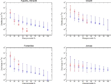
To assess the relative performances of the regionalization procedure for flow estimation in ungauged catchments, usu-ally the simulated flow is compared to the observed one and/or sometimes gauged catchments are considered in turn as if they are ungauged (Oudin et al., 2008). In the cur-rent work, catchments have very scarce streamflow records. Therefore any available observation data, field knowledge and/or previous work conducted in the area of interest can be precious and helpful to check the performance of the adopted regionalization method. Performance assessment of the re-gionalization procedure is based on three evaluation crite-ria. The first one is namely fit to observation (van Griensven et al., 2012) and consists of the quantitative assessment of model accuracy simulations compared to measurements us-ing some statistical criteria. In this regard, the simulated FDC flow percentiles are compared to the observed ones by using the NS coefficient, and the model prediction uncertainty is

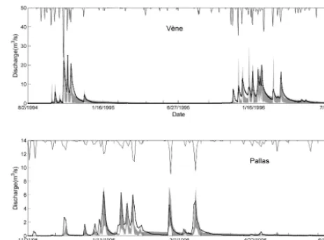
Figure 3. GLUE prediction uncertainty bounds for the Vène and

the Pallas catchment. The grey shaded area is the 95 % prediction uncertainty interval and the black dotted line corresponds to the ob-served discharge.

assessed through thep factor (percentage of observed data bracketed in the 95 % uncertainty interval) wherever obser-vation data are available. The second one is called fit to real-ity (van Griensven et al., 2012) and consists of the evaluation of the model capability in reproducing the real hydrological process and in reflecting the reality of the field. For instance, the predicted mass balance can be calculated and used to assess the performance of the regionalization procedure in representing the main hydrological processes that govern the hydrology of the study system. The third evaluation crite-rion is called fit to geography and it consists of mapping the predicted variable in order to check the soundness of its spa-tial distribution with some observed data (e.g., soil moisture maps) or with some field knowledge (e.g., geology, karstic system, etc.).

5 Results and discussions

5.1 Model performances and prediction uncertainty at the gauged catchments

The NS values range from 0 to 0.71, with an average value of 0.47 for the Vène catchment, while they range from 0 to 0.76 with an average value of 0.60 for the Pallas catchment. The coefficient (R2)is higher than 0.80 in both catchments, indi-cating that SWAT is able to satisfactorily reproduce the gen-eral behavior of the observed hydrograph of both watersheds. The GLUE parameter sets are more robust and consistent in providing simulations that better match the observations of the Pallas catchment than these of the Vène catchment.

bracketed by this interval is estimated using the p factor. The 95 % GLUE uncertainty interval for the Vène and the Pallas catchments is plotted in Fig. 3. The ASRIL and the

p factor are 2.48 and 70 % for the Pallas catchment, while the same statistics are 2.75 and 63 % for the Vène catch-ment, respectively. The statistics are far from their suggested values (ASRIL≈0 andp factor≈100 %), indicating wide prediction uncertainty for both catchments. The reasons can be attributed to several uncertainty sources (e.g., input data, parameter uncertainty, model structure uncertainty, error in the measured data, etc.) and to the subjectivity in the GLUE method (e.g., threshold value, the likelihood function, the ini-tial parameter distribution) involved at each modeling step (Xiong and O’Connor, 2008; Shrestha et al., 2009). Further-more, the karstic nature of the study site (especially the Vène catchment) makes the discharge modeling using the SWAT model more challenging and more uncertain (Sellami et al., 2013).

Besides the model prediction uncertainty, the parameters correlation and posterior distribution are investigated (results not shown). It is noted that different GLUE parameter com-binations lead to similar model results in both case studies. This is known as the equifinality concept (Beven and Bin-ley, 1992) which is behind the GLUE method philosophy. Equifinality originates from the imperfect knowledge of the system under consideration and from different error sources (errors in input and boundaries conditions, errors in using an approximate model structure of the real system and error in the observation variable being modeled) that can interact in a non-linear way (Beven, 2006). In addition, some parameters depicted as very sensitive by the SA method turned out to be less sensitive or less important by the GLUE method, such as ALPHA_BF and GWQMN. In fact, given the equifinality behind the GLUE concept and the possible correlations and interactions between parameters, a single parameter may lose in importance in the context of a combination of parameters values. As a corollary, GLUE cannot reveal the sensitivity of a single parameter.

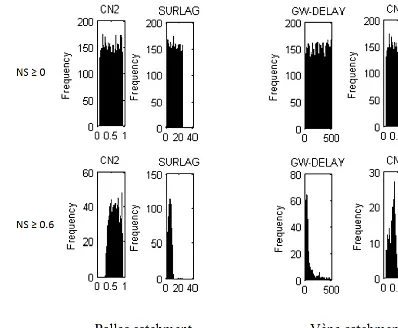
The posterior parameters distribution (PDs) derived from the Monte Carlo runs are large and rather uniformly dis-tributed over their range. This is because GLUE tends to flatten the response surface of the parameter by giving equal weight to “behavioral” model runs. These results are consis-tent with previous studies (e.g., Yang et al., 2008; Dotto et al., 2012). However, the PDs shape and the uncertainty range of the parameters are dependent on the selected threshold value (Fig. 4). By selecting a threshold NS≥0, all parameters are rather uniformly distributed, which lead to non-identifiable parameters indicating wide parameter uncertainty. While in-creasing the threshold value to NS=0.60, some parame-ter PDs become narrower and peakier and well identified. This is illustrated in Fig. 4 for the example of the CN2 and GW_DELAY for the Vène catchment, and CN2 and SURLAG parameters for the Pallas catchment. In addition to the shape of the parameter PDs, increasing the

thresh-Figure 4. Example of the effect of the threshold value on the

poste-rior parameter distribution derived from GLUE.

old value results in a decline of the numbers of “behavioral” Mps retained and causes the depletion of the coverage of the observation by the uncertainty interval. For instance, by se-lecting a threshold value NS≥0.60, thep factor decreased from 70 to 46 % and from 63 to 53 % for the Pallas and the Vène catchments, respectively. The ASRIL also decreased to 2.23 and to 1.92 in the Vène and in the Pallas catchments, respectively, following the increase of the threshold value. These results are in accordance with the findings of Blasone et al. (2008) and Gong et al. (2011) and suggest that interpre-tation of parameter uncertainty derived by GLUE is always conditioned to the choices of threshold value and the predic-tion uncertainty level.

Investigations of the parameters correlation matrices (data not shown) show very low correlation between the param-eters. It seems that GLUE does not explicitly account for parameters interaction. Many authors (Blasone et al., 2008; Yang et al., 2008; Jin et al., 2010) have reported the weak cor-relation between parameters within the GLUE method. One explanation can be that the selected sampling strategy can-not account for parameter interaction since each parameter is individually and randomly sampled from its distribution. 5.2 Results of the regionalization approach

5.2.1 Catchment clustering

Table 4. Results of catchment clustering and number of Mps transferred from the donor to the receptor catchment based on the similarity

measure.

Donor Receptor Threshold % of

catchment catchment Similarity (Thresh) Mps

Catchments

cluster Vène Joncas 0.71 0.50 44.10

Lauze 0.70 0.49 46.95

Aiguilles 0.66 0.46 54.62

Mayroual 0.36 0.25 89.18

Pallas Nègues_Vacques 0.88 0.66 16.60

Aygues_Vacques 0.71 0.54 85.16

Soupié 0.70 0.53 86.47

Fontanilles 0.50 0.38 96.52

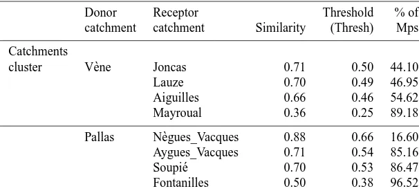
Note: the %Mps corresponds to the percentage of the transferred Mps out of 10 000.

are identified as the donor catchments while all the other un-gauged watersheds are considered as receptor catchments. The highest threshold value (Thresh) calculated using Eq. (3) is Thresh=0.50 and 0.66 for the Vène and the Pallas catch-ment, respectively. These Thresh values are frequently used in the literature to identify “behavioral” Mps (Gassman et al., 2007; Shen et al., 2012). The lowest Thresh values range be-tween 0.25 and 0.38, corresponding to a transfer of 89.18 % and of 96.52 % of the total Mps sets of the Vène and the Pal-las catchments, respectively (Table 4). These Thresh values correspond to poor model performances at the gauged catch-ments and can be seen as low compared to what has been usu-ally used in literature. However, as it was reported by Oudin et al. (2008), it is not straightforward to state whether or not poorly modeled gauged catchment(s) parameters should be transferred to ungauged catchment(s). On the one hand, it is expected that Mps associated with poorly modeled hydro-graphs in gauged catchment(s) will yield poor model per-formances at the ungauged catchment(s). On the other hand, transfer of Mps from poorly modeled gauged catchment(s) may add an element of diversity, which can be beneficial for modeling the ungauged catchment (Oudin et al., 2008).

5.2.2 Predicted flow duration curves (FDCs) at the ungauged catchments

The FDC provides the percentage of time (duration) a daily or monthly (or some other time interval) streamflow is ex-ceeded over a period for a particular river basin (Castel-larin et al., 2004). FDC may also be viewed as the comple-ment of the cumulative distribution function of the consid-ered streamflow and is probably one of the most informative methods of displaying the complete range of river discharges, from low flows to flood events. Empirical FDCs can be easily constructed from streamflow observations using standardized non-parametric procedures (see Vogel and Fennessey, 1994, 1995; Smakhtin, 2001; Castellarin et al., 2004). The FDC concerns only the flow magnitude, whereas the streamflow

time series concerns both magnitude and time sequence. The flow percentiles conceptually represent different segments of the FDC: high flow (≤Q10), median flows (Q10–Q50) and low flows (Q50–Q100). The simulated FDCs resulting from the transfer of the GLUE Mps sets of the Pallas and Vène catchments to the ungauged catchments (within their corre-sponding group) are plotted in Fig. 5.

Figure 5. Simulated uncertain FDCs for the ungauged catchments

based on model parameters regionalization.

in both catchment group do not exceed 0.015 m3s−1. How-ever, the variation in the mean values of the simulated FDCs is more important in high flow percentiles than in low flow percentiles in both catchment groups. In the Pallas catch-ment group, the mean flow magnitude decreases rapidly from

Q10 to Q20, then progressively from Q20 to Q50, leading to a progressive increase in the CV within these flow per-centiles. It also tends to be steady for flow percentile higher thanQ50, which results in higher CV values. In addition, at low flow percentiles (> Q50), all the simulated FDCs of the Pallas catchment group tend to have similar mean flow val-ues, which resulted in less variability of the CV at the low flow percentiles. Also, catchments within the Vène group have much more variability in their simulated flow percentile mean values than those of the Pallas group. The flow per-centiles of the simulated FDCs of the Aiguilles catchment have the highest mean values, while the Mayroual and Lauze

Table 5. Measure of the ASRIL factor of the predicted FDC

uncer-tainty intervals in the ungauged catchments.

Ungauged catchment Donor catchment

Vène Pallas

Lauze 0.018 –

Aiguilles 0.031 –

Joncas 0.019 –

Mayroual 0.207 –

Fontanilles – 0.196

Aygues_Vacques – 0.117

Nègues_Vacques – 0.113

Soupié – 0.169

FDC flow percentiles are very similar and those of the Joncas catchment are the lowest values. It is worth noting here that the CV of low flow percentiles is also compared to the catch-ment drainage area and to the soil characteristics within each ungauged catchment, but no clear relationships is found. 5.2.3 Uncertainty in the predicted FDCs at the

ungauged catchments

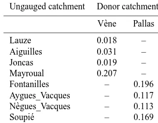
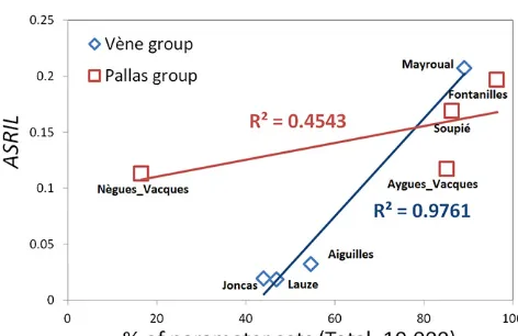
The uncertainty in simulated FDCs are represented in Fig. 5 in such a way that dissimilarity between the donor and the receptor catchment, within each catchment group, increases from the left to the right and from top to down. It is clearly seen in Fig. 5 that the FDC uncertainty interval in both catch-ment groups is wider, as the receptor catchcatch-ment is further from the donor catchment. This is also confirmed by the re-lationship that exists between the number of Mps transferred from the donor to the receptor catchments and the ASRIL factor plotted in Fig. 7. The ASRIL factor increases as the percentage of the transferred Mps increases. While the av-erage FDC uncertainty width (ASRIL) in both catchment groups tends to increase as the dissimilarity between the donor and the receptor catchments increases, catchments of the Pallas group show a wider uncertainty interval than these of the Vène group. Another observation that can be made from Figs. 5 and 7 is that catchments that are very similar to each other have similar, uncertain FDC shapes and very close ASRIL factor values (see also Table 5). This is the case for the Joncas and Lauze catchments in the Vène group and for the Nègues_Vacques and Aygues_Vacques catchments in the Pallas group. This suggests that high similarity between CAs may lead to similar hydrological responses and model pre-diction uncertainties of catchments that are under the same climatic and geographic region. However, this assumption is far from being validated in this work and needs to be further investigated and checked in future work with a larger number of similar catchments or by simply gauging the catchments.

Figure 6. Mean and coefficient of variation of the predicted FDC percentiles based on the physical similarity approach for the Pallas

catchment group (Pallas) and for the Vène catchment group (Vène).

Figure 7. Relationship between the number of transferred model

parameter sets and the ASRIL factor at the ungauged catchments.

catchment and the predicted uncertainty of the FDCs in the receptor catchments exist. This has been done through the calculation of the coefficient of variation (CV) of the trans-ferred Mps within each ungauged catchment. The CV, as it was described previously, can be used as a dimensionless measure of parameter uncertainty (Bastola et al., 2008). The variability of the CV of Mps transferred to the ungauged catchments within each catchment group is given in Fig. 8. Results show that the CV of Mps varies between the

catch-ments, depending on the parameter itself and on the similar-ity distance between the receptor and the donor catchments.

Figure 8. Relationship between the CV variability of the transferred

model parameter from gauged to the ungauged catchments and the ASRIL factor within each catchment group.

the transferred parameter uncertainty and the predicted un-certainty width of the FDCs and between the CAs similarity distance and the predicted uncertainty in the ungauged catch-ment. The results are consistent with the proposed methodol-ogy in this work, which is based on the principle that model prediction uncertainty intuitively increases as the dissimilar-ity in CAs between the donor and the receptor catchments increases. However, these results need to be interpreted with care and precaution. Indeed, the CV is calculated for each model parameter individually without simultaneously taking into account the uncertainty and the interactions between the other parameters, while it is the whole parameter set that was transferred in the regionalization schemes. By relating the parameter CV to the model prediction uncertainty in un-gauged catchment, it is assumed that a linear relationship ex-ists between parameter uncertainty and model prediction un-certainty at the ungauged catchments. However, this linear-ity is difficult to check and to establish because of the pos-sible interdependency of the parameters, non-linearity and non-monotonicity of the hydrological model and other var-ious sources of uncertainty (uncertainty in input and model structure). Moreover, model parameters that have steady CV across the ungauged catchments may contribute to model

Table 6. Statistical criteria of the regionalization approach results.

Aygues_

Catchment Vacques Soupié Fontanilles Joncas

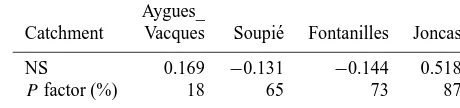
NS 0.169 −0.131 −0.144 0.518

P factor (%) 18 65 73 87

prediction uncertainty when they are transferred in a set of parameters. Therefore, the CV of an individual parameter may not reflect its real uncertainty. In addition to Mps, input and model structure uncertainty, regionalization procedures are known to have additional uncertainty on model prediction in ungauged catchments (Wagener et al., 2004; Heuvelmans et al., 2006; Bastola et al., 2008). In the proposed methodol-ogy it is assumed that uncertainty that stems from the region-alization schemes is propagated to model prediction in the ungauged catchment through the integration of the similarity measure in defining the Mps sets to be transferred from the donor to the receptor catchments. However, partitioning each uncertainty source and telling to which extent it can affect the model prediction is a very difficult task to perform.

5.3 Performances evaluation of the regionalization approach

5.3.1 Fit to observation

Figure 9. The 95 % uncertainty interval of the simulated FDC flow percentiles versus 95 % of the observed FDC flow percentiles

re-sulting from the model parameters regionalization approach. Results correspond to the transfer of the Pallas model parameter sets to the Aygues_Vacques, Soupié and Fontanilles catchments and transfer of the Vène model parameter sets to the Joncas catchments. The blue color is for simulation and the red color is for observation. The bar corresponds to the 95 % flow percentile value, while the square corresponds to the flow percentile median value.

tendency of the p factor increase with the decrease of the distance between the donor and the receptor catchment. As was demonstrated previously, the average relative width of the uncertainty interval (ASRIL) increases as the dissimilar-ity between the donor and the receptor catchments increases. Therefore, more observation data are bracketed in the flow percentile uncertainty interval of the ungauged catchments that are located far from the donor catchment.

5.3.2 Fit to reality

The annual mass balance is calculated based on the average annual values of the different hydrological components that are computed by the SWAT model according to Eq. (6). WYLD=Surf_Q+Lat_Q+GW_Q−TLosses, (6) where WYLD is the net water yield to reach (mm), Surf_Q

is the surface runoff (mm), Lat_Qis the lateral flow contri-bution to reach (mm), GW_Qis the groundwater discharge into the reach (mm) andT Losses is the amount of water re-moved from the tributary channel by transmission (mm). The WYLD decomposes the contribution of the different flow types to the total water budget and is actually equal to pre-cipitation diminished by evapotranspiration.

The average annual water budget, its components and their corresponding uncertainty (calculated as the standard devi-ation) for each ungauged catchment are plotted in Fig. 10. The results of the regionalization approach suggest that sur-face runoff is the major component of the water budget (65 % on average) followed by the lateral flow (22.7 % on average) and by the groundwater flow (12.3 % on average). However, all the hydrological balance components are estimated with large uncertainty. For instance, about 65 % of the WYLD uncertainty is attributed to the uncertainty of the estimated surface runoff (Surf_Q). In the SWAT model, Surf_Qis es-timated using the modified Soil Conservation Service (SCS) curve number (CN) method, which depends on the soil mois-ture and land use cover. Therefore, any uncertainty in the soil and land use cover is translated to the associated curve num-ber and affects the predicted Surf_Q. Moreover, in SWAT the runoff coefficient is calculated as the ratio of runoff vol-ume to rainfall. Therefore, uncertainty of the latter can affect the predicted peak flow, which in turn affects the predicted Surf_Q.

Figure 10. Average annual water balance simulated at the ungauged

catchments based on the regionalization approach. The error bars represent the standard deviation calculated based on all model sim-ulations.

Pallas catchment group (Nègues_Vacques, Aygues_Vacques, Soupié and Fontanilles), with an average of 6.47 %. In addi-tion, GW_Qwithin the Pallas catchment group occurs inter-mittently, while it seems more sustained but also more uncer-tain within the Vène catchment group (Fig. 10). Because of the different sources of uncertainty (e.g., precipitation, evap-otranspiration, uncertainty in groundwater parameters) and the rainfall seasonal variability, the groundwater volume and its level of fluctuation are estimated with uncertainty that is translated into an uncertain GW_Q. These results suggest that streamflow in the Vène catchment group (corresponding more or less to the eastern part of the Thau catchment, see Fig. 1) is more influenced by the groundwater flow contribu-tion than in the Pallas catchment group (corresponding to the central and western part of the Thau catchment). However, the validation of this result is not straightforward since no in-formation or data on groundwater are available in the study area and more hydrogeological measurements are required to check the results and to reduce the groundwater discharge uncertainty.

About 2.5 % of the total water budget is lost via leach-ing through the stream bed (T Losses). This type of losses is more important in the Pallas catchment group (5.3 %), than in the Vène catchment group (1.37 %) (Fig. 10). Transmis-sion losses become more important when GW_Qdecreases and vice versa. Because the SWAT model creates a more sus-tained shallow aquifer with larger water storage in the eastern part than in the western part of the Thau catchment, the Vène catchment group gain much more water through baseflow (GW_Q+Lat_Q), leading to smaller loss of water through channel transmission. However, besides the depth of water stored in the shallow aquifer, other geomorphologic parame-ters (e.g., the width and length of the channel bed, etc.) and hydraulic parameters (e.g., effective hydraulic conductivity of the river bed (Ch_K), geologic nature of the channel

ma-terial) can affect the transmission losses amount. For exam-ple, for catchments where the groundwater level is beyond the river bed, the CH_K value should be equal to zero (van Griensven et al., 2012) and should not be too high in hu-mid catchments. Uncertainty in the estimated transmission losses can stem from the uncertainty of the physical features of the catchments introduced through the GIS data and used by SWAT to derive the channel geomorphological character-istics and from the uncertainty of the CH_Kparameter.

5.3.3 Fit to geography

This criterion is used here to assess the performances of the regionalization procedure in reproducing the actual spa-tial distribution of the soil moisture in the Thau catch-ment. Baghdadi et al. (2012) proposed a method to esti-mate the volumetric soil moisture from RADARSAT-2 im-age (space Synthetic Aperture Radar “SAR” sensor) for bare agricultural fields or fields with thin vegetation cover over the Thau Basin for 10 dates between November 2010 and March 2011. Their estimated soil moisture values showed a good agreement with the measured in situ soil moisture, with RMSE=0.065 cm3cm−3 (see Baghdadi et al., 2012 for details). These estimated soil moisture maps, referred to hereafter as observed soil moisture, are compared to the soil moisture derived from the regionalization results, which are referred to hereafter as predicted soil moisture. Since the ob-served soil moisture maps are available only for three dif-ferent dates (18 November, 4 and 12 December 2010) within the model simulation period, the comparison between the ob-served and the predicted soil moisture is restricted to these three dates. Figure 11 shows the spatial distribution of the predicted and the observed soil moisture for three different dates at the Thau catchment. The predicted soil moisture is spatially correlated to the observed one, but with a different degree of satisfaction. The latter can be broadly and arbitrar-ily set to good, satisfactory or poor based on the graphical investigation of Fig. 11. Good spatial correlation between the distribution of the predicted and the observed soil moisture is obtained at the Vène, Aiguilles and Fontanilles catchments, while it can be considered as satisfactory for the Joncas, Lauze, Pallas and Soupié and poor for the Aygues_Vacques, Mayroual and Nègues_Vacques catchments. Overall, the pre-dicted soil moisture has an acceptable spatial distribution with the observed one, which is more clear in the eastern part (corresponding to the Vène catchment group) than in the western part (corresponding to the Pallas catchment group) of the Thau catchment.

Figure 11. Distribution of the soil moisture within the Thau catchment for three different dates; (a) is the observed soil moisture (Baghdadi

et al., 2012) and (b) is the predicted soil moisture based on the regionalization results.

Table 7. Statistical criteria of the 95 % confidence observed and predicted soil moisture values on the three dates at the Thau catchment.

Observed soil moisture (cm3cm−3) Predicted soil moisture (cm3cm−3)

Date 18 Nov 2010 4 Dec 2010 12 Dec 2010 18 Nov 2010 4 Dec 2010 12 Dec 2010

Prec.* min–max 2.2 0.08–0.27 0.6 0.10–0.26 0 0.03–0.19 2.2 0.08–0.33 0.6 0.04–0.30 0 0.01–0.28

Median 0.167 0.162 0.07 0.142 0.102 0.07

Mean 0.169 0.166 0.08 0.167 0.127 0.09

Note: * Prec. is the cumulative precipitation in (mm) from the 3 previous days to the selected date.

when this day is preceded by wet days (Table 7). Neverthe-less, the median and the mean of the observed and predicted soil moisture values are in good agreement. However, the comparison of the observed and predicted soil moisture val-ues is not straightforward, since the model predicts the soil moisture at the HRU scale for soils with different vegetation-type cover, while the observed soil moisture values are made up for bare soils or soils with thin vegetation cover. In addi-tion, observed soil moisture values are made up for the top 5 to 10 cm of the soil profile, whereas the predicted ones might be estimated by SWAT for the entire soil layer, which can be much more than 10 cm depth.

6 Summary and conclusions

We first questioned whether the selected hydrological model is suitable for reproducing the hydrology of the study area. The model showed good performances in reproducing the daily observed discharge of the Vène and the Pallas catch-ments with NS coefficient higher than 0.70. The model was able to cover more than 60 % of the observation discharge data of each catchment in its 95 % prediction uncertainty in-terval. However, the model prediction uncertainty was large in both study sites, especially in the Vène catchment.

We subsequently questioned whether the selected hydro-logical model is able to predict the discharge at ungauged catchments. We analyzed this question through the transfer of the SWAT model parameter sets from the gauged catch-ments (Vène and Pallas) to the ungauged catchcatch-ments of the Thau watershed. A regionalization approach based on sim-ilarity measure between catchments attributes was adopted to identify similar catchments clusters. Within each cluster, the degree of similarity between the donor and the receptor catchment was used as a threshold to select the appropriate transferrable model parameter sets.

Results showed that within the same catchments cluster, ungauged catchments can exhibit similar hydrologic behav-ior if they exhibit high degree of similarity in their physi-cal attributes and have received similar model parameter sets. Similar ungauged catchments showed higher similarity at the predicted FDC high flow percentiles than at low flow per-centiles. The high variability of the predicted low flow val-ues was attributed to the predicted low mean valval-ues of the flow percentiles rather than to the geology or to the catch-ment drainage area.

The performance of the regionalization method at the un-gauged catchments was assessed through statistical and field reality criteria. The predicted median flow percentiles, given the available observed data, were poorly to acceptably repro-duced by the model. The predicted water balance revealed the prevailing of the surface runoff component in the hydrol-ogy of the ungauged catchments. The predicted soil moisture was satisfactorily spatially correlated to the observed one for some given dates. The findings suggest that the SWAT model parameters can be regionalized to predict discharge at un-gauged catchments and the results can fit the reality of the case study. However, thorough evaluation and criticism of its performances is constrained by the availability of the ob-servation data at the ungauged catchments. Therefore, other evaluation criteria such as fit to reality and fit to geography can be used to describe the model performances in these un-gauged catchments.

We also showed in this work how parameter uncertainty can affect model prediction uncertainty at ungauged catch-ments through the regionalization of the model parameters. The assumptions behind the developed methodology were that physically similar catchments are hydrologically similar and model prediction uncertainty increases as the dissimilar-ity between the donor and the receptor catchment increases. The developed methodology allows propagating model

pa-rameter uncertainty proportionally to the similarity measure. Furthermore, it makes the selection of the donor catchment parameter sets more objective than the traditional approach, which is based on modeler subjective choice. It was shown that model prediction uncertainty was influenced by the simi-larity distance between the donor and the receptor catchment. Wider prediction uncertainty is obtained as the dissimilarity between the donor and the receptor catchment increases. It was also shown that within the same climatic and geographic region, catchments that are very similar to each other and have received similar model parameter sets exhibit a sim-ilar degree of prediction uncertainty. In addition, the find-ings showed that the selected threshold values and, hence, the number and the uncertainty of the parameters transferred can affect the prediction uncertainty at the ungauged catchment. If a higher degree of similarity exists between the donor and the receptor catchments then a higher threshold value is se-lected. Consequently, a lower parameter uncertainty is propa-gated to the ungauged catchment, leading to lower prediction uncertainty in the ungauged catchment. Otherwise, a lower threshold value is selected and wider uncertain parameter sets are transferred, which will yield a larger uncertain model prediction at the target catchment. However, these results do not pretend that uncertainty in the transferred parameter sets is the only source for model prediction uncertainty at the un-gauged catchment. As it was demonstrated by the results, al-though the relationship between uncertainty in the parame-ters and in the prediction results at the ungauged catchments exists, this relationship is too far to be linear. This is due to other sources of uncertainty (e.g., model structure, inputs un-certainty), parameter correlation and equifinality. Therefore, all sources of uncertainty should be considered in an inte-grated framework for more effective parameter regionaliza-tion.

To our knowledge, a hydrological study of the entire Thau catchment has never been done before. Therefore, building on the regionalization approach, this work can be considered as a starting point for further research study of hydrological issues in this catchment.

estimating flow at ungauged catchments within an uncer-tainty propagation framework.

Acknowledgements. This work was funded by the IDB (Islamic Development Bank) under its Ph.D. Merit Scholarship program. The work has been conducted in the context of the European project CLIMB (Climate induced changes on the hydrology of Mediterranean Basins, http://www.climb-fp7.eu/home/home.php). Authors thank Egis eau, the Syndicat Mixte du Bassin du Thau and Ifremer for providing most of the data.

Edited by: A. Shamseldin

References

Abbaspour, K. C., van Genuchten, M. T., Schulin, R., and Schläppi, E.: A sequential uncertainty domain inverse procedure for esti-mating subsurface flow and transport parameters, Water Resour. Res., 33, 1879–1892, doi:10.1029/97wr01230, 1997.

Aquilina, L., Ladouche, B., Doerfliger, N., Seidel, J. L., Bakalow-icz, M., Dupuy, C., and Le Strat, P.: Origin, evolution and res-idence time of saline thermal fluids (Balaruc springs, south-ern France): implications for fluid transfer across the con-tinental shelf, Chem. Geol., 192, 1–21, doi:10.1016/S0009-2541(02)00160-2, 2002.

Arabi, M., Govindaraju, R. S., and Hantush, M. M.: A proba-bilistic approach for analysis of uncertainty in the evaluation of watershed management practices, J. Hydrol., 333, 459–471, doi:10.1016/j.jhydrol.2006.09.012, 2007.

Arnold, J. G., Srinivasan, R., Muttiah, R. S., and Williams, J. R.: Large area hydrological modeling and assessment Part I: Model development 1, J. Am. Water. Resour. Ass., 34, 73–89, doi:10.1111/j.1752-1688.1998.tb05961.x, 1998.

Baghdadi, N., Cresson, R., El Hajj, M., Ludwig, R., and La Je-unesse, I.: Estimation of soil parameters over bare agriculture ar-eas from C-band polarimetric SAR data using neural networks, Hydrol. Earth Syst. Sci., 16, 1607–1621, doi:10.5194/hess-16-1607-2012, 2012.

Bàrdossy, A.: Calibration of hydrological model parameters for ungauged catchments, Hydrol. Earth Syst. Sci., 11, 703–710, doi:10.5194/hess-11-703-2007, 2007.

Bastola, S., Ishidaira, H., and Takeuchi, K.: Regionalisation of hydrological model parameters under parameter uncertainty: A case study involving TOPMODEL and basins across the globe, J. Hydrol., 357, 188–206, doi:10.1016/j.jhydrol.2008.05.007, 2008.

Beven, K. J.: TOPMODEL: a critique, Hydrol. Process., 11, 1069– 1086, 1997.

Beven, K.: On the future of distributed modelling in hydrology, Hy-drol. Process., 14, 3183–3184, doi:10.1002/1099-1085, 2000. Beven, K.: A manifesto for the equifinality thesis, J. Hydrol., 320,

18–36, doi:10.1016/j.jhydrol.2005.07.007, 2006.

Beven, K. and Binley, A.: The future of distributed models: Model calibration and uncertainty prediction, Hydrol. Process., 6, 279– 298, 1992.

Beven, K. and Freer, J.: Equifinality, data assimilation, and uncer-tainty estimation in mechanistic modelling of complex environ-mental systems using the GLUE methodology, J. Hydrol., 249, 11–29, 2001.

Blasone, R.-S., Madsen, H., and Rosbjerg, D.: Uncertainty assess-ment of integrated distributed hydrological models using GLUE with Markov chain Monte Carlo sampling, J. Hydrol., 353, 18– 32, doi:10.1016/j.jhydrol.2007.12.026, 2008.

Castellarin, A., Galeati, G., Brandimarte, L., Montanari, A., and Brath, A.: Regional flow-duration curves: reliability for ungauged basins, Adv. Water Resour., 27, 953–965, doi:10.1016/j.advwatres.2004.08.005, 2004.

Chahinian, N., Tournoud, M.-G., Perrin, J.-L., and Picot, B.: Flow and nutrient transport in intermittent rivers: a modelling case-study on the Vène River using SWAT 2005, Hydrol. Sci. J., 56, 268–287, doi:10.1080/02626667.2011.559328, 2011.

Dotto, C. B., Mannina, G., Kleidorfer, M., Vezzaro, L., Henrichs, M., McCarthy, D. T., Freni, G., Rauch, W., and Deletic, A.: Com-parison of different uncertainty techniques in urban stormwa-ter quantity and quality modelling, Wastormwa-ter Res., 46, 2545–2558, doi:10.1016/j.watres.2012.02.009, 2012.

Duan, Q., Sorooshian, S., and Gupta, V.: Effective and efficient global optimization for conceptual rainfall-runoff models, Water Resour. Res., 28, 1015–1031, doi:10.1029/91wr02985, 1992. Eckhardt, K., Fohrer, N., and Frede, H.-G.: Automatic model

cal-ibration, Hydrol. Process., 19, 651–658, doi:10.1002/hyp.5613, 2005.

Freer, J., Beven, K., and Ambroise, B.: Bayesian Estimation of Un-certainty in Runoff Prediction and the Value of Data: An Applica-tion of the GLUE Approach, Water Resour. Res., 32, 2161–2173, doi:10.1029/95WR03723, 1996.

Freni, G. and Mannina, G.: Bayesian approach for un-certainty quantification in water quality modelling: The influence of prior distribution, J. Hydrol., 392, 31–39, doi:10.1016/j.jhydrol.2010.07.043, 2010.

Gallart, F., Amaxidis, Y., Botti, P., CanÈ, G., Castillo, V., Chapman, P., Froebrich, J., GarcÍA-Pintado, J., Latron, J., Llorens, P., Porto, A. L., Morais, M., Neves, R., Ninov, P., Perrin, J.-L., Ribarova, I., Skoulikidis, N., and Tournoud, M.-G.: Investigating hydrolog-ical regimes and processes in a set of catchments with temporary waters in Mediterranean Europe, Hydrol. Sci. J., 53, 618–628, doi:10.1623/hysj.53.3.618, 2008.

Gassman, P. W., Reyes, M. R., Green, C. H., and Arnold, J. G.: The Soil and Water Assessment Tool: Historical development, applications and future research directions, Trans. ASABE, 50, 1211–1250, 2007.

Gitau, M. W. and Chaubey, I.: Regionalization of SWAT Model Pa-rameters for Use in Ungauged Watersheds, Water, 2, 849–871, 2010.

Gong, Y., Shen, Z., Hong, Q., Liu, R., and Liao, Q.: Parameter un-certainty analysis in watershed total phosphorus modeling using the GLUE methodology, Agr. Ecosys. Environ., 142, 246–255, doi:10.1016/j.agee.2011.05.015, 2011.