Multi-objective Optimization of Surface Roughness and Material Removal Rate Using an Improved Self-Adaptive Particle Swarm Optimization Algorithm in Milling process

AUT Journal of Mechanical Engineering

AUT J. Mech. Eng., 2(1) (2018) 117-123 DOI: 10.22060/ajme.2018.12581.5373

Multi-objective Optimization of Surface Roughness and Material Removal Rate Using

an Improved Self-Adaptive Particle Swarm Optimization Algorithm in the Milling

process

M. M. Abootorabi*

Faculty of Mechanical Engineering, Yazd University, P.O.B. 89195-741, Yazd, Iran

ABSTRACT: Surface roughness is one of the main characteristics of a work piece in the quality control process. Several parameters such as cutting tool material and geometry, cutting parameters, work piece material properties, machine tool and coolant type affect the surface quality. An important task of process planners is the proper selection of three main cutting parameters: cutting speed, feed rate, and depth of cut in order to have not only low surface roughness, but also to perform the process within a reasonable amount of time. In this paper, using full factorial experiment design, the multiple regression equation for the surface roughness in the climb milling process of DIN 1.4021 martensitic stainless steel has been obtained and then used as one of the objective functions in the Multi-objective Improved Self-Adaptive Particle Swarm Optimization (MISAPSO) algorithm. This algorithm has been used to obtain cutting parameters to achieve low surface roughness simultaneously with a high material removal rate. The relatively new algorithm MISAPSO developed with some changes in the common particle swarm optimization (PSO) technique, has been used in multi-objective optimization of machining processes and was shown to be able to help the process planners in selecting cutting parameters.

Review History:

Received: 26 February 2017 Revised: 18 December 2017 Accepted: 2 January 2018 Available Online: 15 March 2018

Keywords:

Surface roughness Material removal rate Milling

Regression MISAPSO

117 1- Introduction

Global steel consumption is progressively increasing. In the manufacturing process of a large percentage of parts made of steel, conventional chip removal operations, including milling are used. Martensitic stainless steels, like DIN 1.4021, are widely used in applications for which a combination of high strength and good corrosion resistance is needed such as shear blades and surgical equipment. One of the main challenges that the process planner faces to achieve a high quality work piece is the proper selection of cutting parameters. One of the most important factors in the final quality control of a piece is to consider its surface finish. The surface roughness has a great influence on the corrosion resistance and tribological properties of the piece. For this reason, the proper selection of cutting conditions i.e. cutting speed, feed rate and depth of cut is of great significance and remains as an important topic in manufacturing engineering.

Benardos and Vasniakos [1] carried out a comprehensive literature review of the prediction models for surface roughness. They said that the cutting theory-based models are not exact. This is because of that the mechanisms leading to the formation of surface roughness are very complicated and interacting with nature. Due to the nonlinear and intricate relationship between machining outputs, such as cutting force, tool life and surface roughness, and the cutting parameters, models based on experimental data have been widely developed. These models can be classified into two major categories [2]: (i) models that examine the effects of input factors on the response by employing the multiple

regression method and the analysis of variance to establish this relationship; and (ii) artificial intelligence (AI) based models.

Feng and Wang [3] developed a statistical model for the prediction of surface roughness using nonlinear regression method in turning process. Also, they investigated the effect of cutting parameters, tool point angle, cutting time and work piece hardness on the surface roughness. Ozcelik and Bayramoglu [4] presented an empirical model for the estimation of surface roughness in a high-speed milling operation. These researchers found that the first and second order models developed were in a good agreement with the real values.

Aouici et al. [5] determined the influence of cutting speed, feed rate and cutting time on the tool wear and the surface roughness in turning process of X38CrMoV5-1 steel with a CBN tool using ANOVA and the response surface method (RSM). The authors concluded that the feed rate was the most effective factor on the surface roughness. Asilturk and Cunkas [1] used an artificial neural network (ANN) and multiple regression method to analyze the effect of speed, feed, and depth of cut on the surface roughness of AISI 1040 steel. The predicted values were found to be close to the measured values for both developed models, and the feed rate was the dominant factor affecting the surface roughness followed by the depth of cut and cutting speed. Bharathi Raja and Baskar [6] developed a mathematical model for surface roughness prediction using Particle Swarm Optimization (PSO) on the basis of experimental results in the face milling of aluminum. They found that the predicted roughness using PSO technique was in a good agreement with the measured values.

M. M. Abootorabi, AUT J. Mech. Eng., 2(1) (2018) 115-123, DOI: 10.22060/ajme.2018.12581.5373

118 Kivak [7] applied the Taguchi method and regression analysis to evaluate the machinability of Hadfield steel with PVD and CVD coated inserts under dry milling condition. It was shown that the Taguchi method was very successful in the optimization of cutting parameters for having minimum surface roughness and flank wear. Acayaba and Escalona [8] used experimental data to develop predictive models using multiple linear regression (MLR) and ANN methods. They found that the ANNs were better than MLR for predicting surface roughness in turning processes. Moreover, the authors used the suggested ANN as the fitness function in Simulated Annealing (SA) optimization algorithm in order to obtain a group of cutting parameters that lead to a low surface roughness. Hanief and Wani [9] developed a mathematical model to characterize the surface roughness during the running-in wear process. They said that the ANN model can be used to predict the surface roughness with a high accuracy. Gok [10] presented a new approach to minimize the surface roughness and cutting force via multi-objective grey design and response surface analysis in turning of ductile iron. The study concluded that the depth of cut was the dominant property on the surface roughness and cutting forces. Gupta and Kumar [11] modeled the two response variables i.e. surface roughness and material removal rate (MRR) for turning of unidirectional glass fiber reinforced plastics (UD-GFRP) composite using Principal Component Analysis (PCA) and the Taguchi method. The optimum combination of cutting parameters was found for maximum MRR and minimum surface roughness. The obtained results were verified through confirmation experiments.

Particle swarm optimization algorithm has been used in various research fields such as aerodynamic optimization of a horizontal axis wind turbine blade [12] and updating boring bar’s dynamic model [13], but the use of that to optimize the machining processes has been little done in relation to other fields of research. The aim of the present study is to investigate the effects of the cutting parameters i.e. cutting speed, feed rate, and radial depth of cut on the surface roughness and MRR in the milling process of DIN 1.4021 stainless steel. Using the multiple linear regression method an equation has been obtained for surface roughness, and this equation has been used as one of the objective functions in a multi-objective improved self-adaptive particle swarm optimization (MISAPSO) algorithm in order to achieve the cutting parameters that result in a low surface roughness and high material removal rate simultaneously. In this study, the power of the relatively new algorithm MISAPSO which was developed with some changes in the traditional particle swarm optimization method has been investigated in the optimization of cutting parameters. The performance and efficiency of this technique have not yet been studied in the published research works in the field of machining optimization. The process planners can use this procedure for selecting the proper cutting parameters in order to get a minimum surface roughness and maximum MRR.

2- Experimental Work

A cubic sample of DIN 1.4021 martensitic stainless steel was used to conduct the milling experiments without coolant. This steel has a chemical composition of 15%C, 1%Mn, 1%Si, 0.04%P, 0.03S and 12-14%Cr [14]. TiN-coated 4-flute flat end mills from HSS with a diameter of D=10 mm were

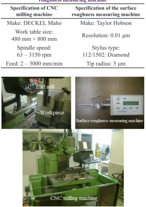
selected for this examination. Once each set of nine tests were carried out on an FP 4 MA CNC milling machine, the work piece was positioned in a bench and a Surtronic 3+ surface roughness measuring machine was used to measure the roughness of the work piece with a cut-off value of 0.8 mm. The surface roughness was measured in the feed direction of the work piece. Figure 1 shows the experimental setup and the surface roughness measuring machine. The specification of CNC milling machine and surface roughness measuring machine have been given in Table 1.

The surface roughness average (R_a) was defined on the basis of the ISO 4287 norm [15] as the arithmetical mean of the deviations of the roughness profile from the central line along the measurement. This definition can be expressed as:

( )

(

)

(

)

(

)

0

2 2 2

2

1

1

. . .

2.65 . .

4.70 0.21 0.55 2.05 0.0032 0.10 1.85 0.0612 . 0.0184 . 0.73 .

1

, ,

ˆ

, ,

: l

a

a r

r

a r

r

r r

n

i i i

a r

r

min

R y x dx

l

MRR N f a a

MRR V f a

R V f a

V f a

V f V a f a

MSE Y Y

n

Minimize R F V f a

Maximize MRR G V f a V

Subject to

=

=

=

=

= − + −

+ − +

+ − −

= −

= = ≤

∫

∑

( )1 ( ) ( )1

min max

max

min max

r r r

t t t

i i i

V V

f f f

a a a

X + X V +

 ≤

 _{≤ ≤}



 _{≤ ≤}



= +

(1)

where y(x) is the coordinate of the roughness profile and l is the evaluation length.

To reduce the effect of noise parameters, the surface roughness was measured three times at different parts of the work piece and their average has been recorded. From the many effective parameters on the surface roughness in milling, the effect of three main cutting parameters, cutting

Specification of the surface roughness measuring machine Specification of CNC

milling machine

Make: Taylor Hobson Make: DECKEL Maho

Resolution: 0.01 μm

Work table size: 480 mm × 800 mm

Stylus type: 112/1502: Diamond Spindle speed:

63 – 3150 rpm

Tip radius: 5 μm

Feed: 2 – 3000 mm/min

Table 1. Specification of CNC milling machine and surface roughness measuring machine

M. M. Abootorabi, AUT J. Mech. Eng., 2(1) (2018) 115-123, DOI: 10.22060/ajme.2018.12581.5373

119 speed (V), feed rate (f ), and radial depth of cut (a_r) were investigated in this study. Levels of cutting parameters have been selected according to the tool, workpiece materials and the tool maker specifications presented in Table 2. Constant cutting conditions in the experiments include an axial cutting depth of a_a= 5 mm and the climb milling process. In climb milling, the cutting tool is fed with the direction of rotation. Figure 2 illustrates schematically the cutting parameters in the climb end milling process.

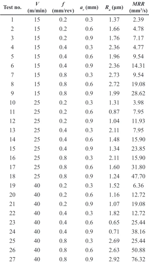
Table 3 shows the cutting parameters and the average surface roughness in each experiment. The full factorial experiment design was selected, and in total, 27 experiments were conducted. Each test was done once.

The material removal rate (MRR) in the end milling process is obtained from the following relationships [16]:

( )

(

)

(

)

(

)

0

2 2 2

2

1

1

. . .

2.65 . .

4.70 0.21 0.55 2.05 0.0032 0.10 1.85 0.0612 . 0.0184 . 0.73 .

1

, ,

ˆ

, ,

: l

a

a r

r

a r

r

r r

n

i i i

a r

r

min

R y x dx

l

MRR N f a a

MRR V f a

R V f a

V f a

V f V a f a

MSE Y Y

n

Minimize R F V f a

Maximize MRR G V f a V

Subject to

=

=

=

=

= − + −

+ − +

+ − −

= −

= = ≤

∫

∑

( )1 ( ) ( )1

min max

max

min max

r r r

t t t

i i i

V V

f f f

a a a

X + X V +

 ≤

 _{≤ ≤}



 _{≤ ≤}



= +

(2) where N is the spindle speed (rpm). By knowing the axial depth of cut a_a=5 mm and the relationship V=πDN, the material removal rate in mm3_{/s becomes:}

( )

(

)

(

)

(

)

0

2 2 2

2

1

1

. . .

2.65 . .

4.70 0.21 0.55 2.05 0.0032 0.10 1.85 0.0612 . 0.0184 . 0.73 .

1

, ,

ˆ

, ,

: l

a

a r

r

a r

r

r r

n

i i i

a r

r

min

R y x dx

l

MRR N f a a

MRR V f a

R V f a

V f a

V f V a f a

MSE Y Y

n

Minimize R F V f a

Maximize MRR G V f a V

Subject to

=

=

=

=

= − + −

+ − +

+ − −

= −

= = ≤

∫

∑

( )1 ( ) ( )1

min max

max

min max

r r r

t t t

i i i

V V

f f f

a a a

X + X V +

 ≤

 _{≤ ≤}



 _{≤ ≤}



= +

(3) This relationship for MRR and the obtained equation for surface roughness that can be found in the following section have been used as the objective functions in the optimization algorithm.

3- Results and Discussion

Based on the experimental data, the multiple linear regression was utilized to model the surface roughness. After ensuring the accuracy of the proposed regression equation, the Multi-objective Improved Self-Adaptive Particle Swarm Optimization (MISAPSO) algorithm was employed to

determine a set of optimum cutting parameters that minimize the surface roughness and maximize the material removal rate.

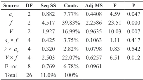
Analysis of variance (ANOVA) can be used to investigate the effect of one or several input parameters on an output parameter or response [17]. In this study, the analysis of variance with the aid of MINITAB software has been done to investigate the effects of input parameters and their interactions on the surface roughness. Table 4 presents the analysis of variance for the surface roughness. According to the performed analysis of variance in Table 3, the amounts of feed rate and cutting speed effect on surface roughness are 39.8% and 17.0%, respectively. The interaction of cutting speed and feed rate has 22.1% effect on the surface roughness.

3- 1- Multiple linear regression

Multiple regression is a method that describes the statistical relationship between a response and two or more independent predictors. Regression often uses the method of least squares, which determines the equation for the straight line that minimizes the sum of the squared vertical distances between

Radial depth of cut (mm) Feed rate

(mm/rev) Cutting speed

(m/min)

0.3 0.2

15

0.6 0.4

25

0.9 0.8

40

Table 2. Cutting Conditions in Experimental Tests

Fig. 2. The cutting parameters in climb end milling process

MRR

(mm3_/s)

R_a (μm)

a_r (mm)

f

(mm/rev)

V

(m/min) Test no.

2.39 1.37

0.3 0.2

15 1

4.78 1.66

0.6 0.2

15 2

7.17 1.76

0.9 0.2

15 3

4.77 2.36

0.3 0.4

15 4

9.54 1.96

0.6 0.4

15 5

14.31 2.36

0.9 0.4

15 6

9.54 2.73

0.3 0.8

15 7

19.08 2.72

0.6 0.8

15 8

28.62 1.99

0.9 0.8

15 9

3.98 1.31

0.3 0.2

25 10

7.95 0.87

0.6 0.2

25 11

11.93 1.04

0.9 0.2

25 12

7.95 2.11

0.3 0.4

25 13

15.90 1.48

0.6 0.4

25 14

23.85 1.34

0.9 0.4

25 15

15.90 2.11

0.3 0.8

25 16

31.80 1.60

0.6 0.8

25 17

47.70 1.24

0.9 0.8

25 18

6.36 1.52

0.3 0.2

40 19

12.72 1.16

0.6 0.2

40 20

19.08 1.07

0.9 0.2

40 21

12.72 1.82

0.3 0.4

40 22

25.44 0.65

0.6 0.4

40 23

38.16 0.71

0.9 0.4

40 24

25.44 2.69

0.3 0.8

40 25

50.88 2.63

0.6 0.8

40 26

76.32 2.92

0.9 0.8

40 27

M. M. Abootorabi, AUT J. Mech. Eng., 2(1) (2018) 115-123, DOI: 10.22060/ajme.2018.12581.5373

120 the data points and the line [18]. Different adjustments were done using MINITAB 14 and the adjustment with the best coefficient of correlation was selected. The suggested regression equation with second-degree that takes into account the interactions of two factors is given by:

( )

(

)

(

)

(

)

0

2 2 2

2

1

1

. . .

2.65 . .

4.70 0.21 0.55 2.05 0.0032 0.10 1.85 0.0612 . 0.0184 . 0.73 .

1 , , ˆ , , : l a a r r a r r r r n i i i a r r min

R y x dx

l

MRR N f a a

MRR V f a

R V f a

V f a

V f V a f a

MSE Y Y

n

Minimize R F V f a

Maximize MRR G V f a V Subject to = = = = = − + − + − + + − − = − = = ≤

∫

∑

( )1 ( ) ( )1

min max

max

min max

r r r

t t t

i i i

V V

f f f

a a a

X + X V +

 ≤  _{≤ ≤}   _{≤ ≤}  = + (4)

The squared multiple correlation coefficient R2 _{and the}

adjusted coefficient R2_{adj of Eq. (4) is 0.714 and 0.563,}

respectively. R2 _{is the percentage of the total variation in}

the response that is explained by input factors in the model. Adjusted R2 _{is a useful tool for comparing linear models with}

different numbers of predictors. The adjusted R2 _increases

only if the new predictor improves the model more than that which would be expected by chance.

The mean squared error (MSE) is a measure of how close a fitted line is to data points. The smaller the MSE, the closer the fit is to the data. If Y is a vector of n predictions, and Y is the vector of observed values, then the MSE of the predictor can be estimated by:

( )

(

)

(

)

(

)

0

2 2 2

2

1

1

. . .

2.65 . .

4.70 0.21 0.55 2.05 0.0032 0.10 1.85 0.0612 . 0.0184 . 0.73 .

1 , , ˆ , , : l a a r r a r r r r n i i i a r r min

R y x dx

l

MRR N f a a

MRR V f a

R V f a

V f a

V f V a f a

MSE Y Y

n

Minimize R F V f a

Maximize MRR G V f a V Subject to = = = = = − + − + − + + − − = − = = ≤

∫

∑

( )1 ( ) ( )1

min max

max

min max

r r r

t t t

i i i

V V

f f f

a a a

X + X V +

 ≤  _{≤ ≤}   _{≤ ≤}  = + (5)

The closer MSE is to 0, the better the proposed model. Here, the value of MSE=0.12 was achieved, which means a good approximation exists for empirical data. The analysis of variance showed that the feed rate ( f ) has the greatest effect on the surface roughness. The main effects plot is shown in Fig. 3.

3- 2- Multi-objective optimization problem

The main aim of this paper is to find the optimum cutting parameters in order to simultaneously maximize the material removal rate and minimize the surface roughness in the milling process. Due to milling machine limitations and the cutting tool manufacturer suggestions, the values of cutting speed, feed rate, and radial depth of cut must be limited between their minimal and maximal experimental values. The multi-objective problem could be written as follows:

( )

(

)

(

)

(

)

0

2 2 2

2

1

1

. . .

2.65 . .

4.70 0.21 0.55 2.05 0.0032 0.10 1.85 0.0612 . 0.0184 . 0.73 .

1 , , ˆ , , : l a a r r a r r r r n i i i a r r min

R y x dx

l

MRR N f a a

MRR V f a

R V f a

V f a

V f V a f a

MSE Y Y

n

Minimize R F V f a

Maximize MRR G V f a V Subject to = = = = = − + − + − + + − − = − = = ≤

∫

∑

( )1 ( ) ( )1

min max

max

min max

r r r

t t t

i i i

V V

f f f

a a a

X + X V +

 ≤  _{≤ ≤}   _{≤ ≤}  = + (6)

In the following, the Multi-objective Improved Self-Adaptive Particle Swarm Optimization (MISAPSO) algorithm is used to solve Eq. (6).

3- 3- MISAPSO Algorithm

Due to the high speed of convergence and also not to settle at the point of local minimum, the PSO method is used in the solution of single-objective and also multi-objective optimization problems. The PSO is a repetitive algorithm that improves its position in each iteration according to the previous position and velocity of the particle, the best previous position of that particle, and the best position among the entire population. The position of the ith particle can be obtained from the following relation:

( )

(

)

(

)

(

)

0

2 2 2

2

1

1

. . .

2.65 . .

4.70 0.21 0.55 2.05 0.0032 0.10 1.85 0.0612 . 0.0184 . 0.73 .

1 , , ˆ , , : l a a r r a r r r r n i i i a r r min

R y x dx

l

MRR N f a a

MRR V f a

R V f a

V f a

V f V a f a

MSE Y Y

n

Minimize R F V f a

Maximize MRR G V f a V Subject to = = = = = − + − + − + + − − = − = = ≤

∫

∑

( )1 ( ) ( )1

min max

max

min max

r r r

t t t

i i i

V V

f f f

a a a

X + X V +

 ≤

 _{≤ ≤}



 _{≤ ≤}



= + (7)

where t is the current iteration, and X_i(j) _{and V}

i(j) are the

position and velocity of the ith particle in the jth iteration, respectively. The velocity V_i(t+1) _{can be obtained as follows:}

( ) ( )

_{( )}

(

( )

)

( )

(

( )

)

(

)

( )

1 1 1 2 2 1 2 1 1 0 . . . . . . .

, , , , 0,1 , 2, ,

4 1 , 1, 2, ,

0,1 , 0.25, 0 i

t t t

i i best i

t best i max min max max j new i n

i i i i _n choas

j j j

i i i

j j

i

V V c rand P X

c rand G X

Iter Iter

cx

cx cx cx cx i N

cx cx cx j n

cx cx ω ω ω ω ω ω ω + − × + = + + − − = − × = ×   =_ … _ = … = × × − = … ∈ ∉

{

}

( )

[

]

( ) ( )

( )

( )

( )

{

} ( )

( )

{

} ( )

( )

0 1 2 1 2 1 2 1 2 .5, 0.75 . , , , , ,

0 1, 2, , :

0 1, 2,

1, 2, , , 1, 2, , , j p i eq i ueq j j k k cx rand

X Cutting parameters c c

Minimize f X f X f X

g X i N

Subject to

h X i N

j p f X f X

k p f X f X

=

=

…

< = …



 _{= = …}



∀ ∈ … ≤

∃ ∈ … <

(8)

where ω is the inertia weight, c₁ and c₂ are learning factors,

rand₁(.) and rand₂(.) are two random values between (0, 1),

P_besti is the best previous experience of the ith particle, and

G_best is the best experience among the entire population. The inertia weight (ω) can be calculated from the following relation: ( ) ( )

_{( )}

(

( )

)

( )

(

( )

)

(

)

( )

1 1 1 2 2 1 2 1 1 0 . . . . . . .

, , , , 0,1 , 2, ,

4 1 , 1, 2, ,

0,1 , 0.25, 0 i

t t t

i i best i

t best i max min max max j new i n

i i i i _n choas

j j j

i i i

j j

i

V V c rand P X

c rand G X

Iter Iter

cx

cx cx cx cx i N

cx cx cx j n

cx cx ω ω ω ω ω ω ω + − × + = + + − − = − × = ×   =_ … _ = … = × × − = … ∈ ∉

{

}

( )

[

]

( ) ( )

( )

( )

( )

{

} ( )

( )

{

} ( )

( )

0 1 2 1 2 1 2 1 2 .5, 0.75 . , , , , ,

0 1, 2, , :

0 1, 2,

1, 2, , , 1, 2, , , j p i eq i ueq j j k k cx rand

X Cutting parameters c c

Minimize f X f X f X

g X i N

Subject to

h X i N

j p f X f X

k p f X f X

=

=

…

< = …



 _{= = …}



∀ ∈ … ≤

∃ ∈ … <

(9)

where ω_max and ω_min are initial and final weights, respectively,

Source DF Seq SS Contr. Adj MS F P

a_r 2 0.882 7.77% 0.4408 4.59 0.047

f 2 4.517 39.83% 2.2586 23.51 0.000

V 2 1.927 16.99% 0.9635 10.03 0.007

a_r × f 4 0.425 3.75% 0.1063 1.11 0.417

V × a_r 4 0.320 2.82% 0.0798 0.83 0.542

V × f 4 2.503 22.07% 0.6257 6.51 0.012

Error 8 0.769 6.78% 0.0961

Total 26 11.096 100%

Table 4. Analysis of variance for the surface roughness

^

M. M. Abootorabi, AUT J. Mech. Eng., 2(1) (2018) 115-123, DOI: 10.22060/ajme.2018.12581.5373

121 Itermax is the maximum iteration number and Iter is the current iteration number.

The MISAPSO algorithm has been used to overcome local optima problems in this study [19]. In MISAPSO, a chaotic improvement had been proposed to introduce a new inertia weight parameter, as seen below:

( ) ( )

_{( )}

(

( )

)

( )

(

( )

)

(

)

( )

1 1 1 2 2 1 2 1 1 0 . . . . . . .

, , , , 0,1 , 2, ,

4 1 , 1, 2, ,

0,1 , 0.25, 0 i

t t t

i i best i

t best i max min max max j new i n

i i i i _n choas

j j j

i i i

j j

i

V V c rand P X

c rand G X

Iter Iter

cx

cx cx cx cx i N

cx cx cx j n

cx cx ω ω ω ω ω ω ω + − × + = + + − − = − × = ×   =_ … _ = … = × × − = … ∈ ∉

{

}

( )

[

]

( ) ( )

( )

( )

( )

{

} ( )

( )

{

} ( )

( )

0 1 2 1 2 1 2 1 2 .5, 0.75 . , , , , ,

0 1, 2, , :

0 1, 2,

1, 2, , , 1, 2, , , j p i eq i ueq j j k k cx rand

X Cutting parameters c c

Minimize f X f X f X

g X i N

Subject to

h X i N

j p f X f X

k p f X f X

=

=

…

< = …



 _{= = …}



∀ ∈ … ≤

∃ ∈ … <

(10) where cx_ij _{is the jth chaotic variable and can be obtained from}

the following relationship [20]:

( ) ( )

_{( )}

(

( )

)

( )

(

( )

)

(

)

( )

1 1 1 2 2 1 2 1 1 0 . . . . . . .

, , , , 0,1 , 2, ,

4 1 , 1, 2, ,

0,1 , 0.25, 0 i

t t t

i i best i

t best i max min max max j new i n

i i i i _n choas

j j j

i i i

j j

i

V V c rand P X

c rand G X

Iter Iter

cx

cx cx cx cx i N

cx cx cx j n

cx cx ω ω ω ω ω ω ω + − × + = + + − − = − × = ×   =_ … _ = … = × × − = … ∈ ∉

{

}

( )

[

]

( ) ( )

( )

( )

( )

{

} ( )

( )

{

} ( )

( )

0 1 2 1 2 1 2 1 2 .5, 0.75 . , , , , ,

0 1, 2, , :

0 1, 2,

1, 2, , , 1, 2, , , j p i eq i ueq j j k k cx rand

X Cutting parameters c c

Minimize f X f X f X

g X i N

Subject to

h X i N

j p f X f X

k p f X f X

=

=

…

< = …



 _{= = …}



∀ ∈ … ≤

∃ ∈ … <

(11)

where N_choas is the number of individuals, n is the number of surge arrester models parameters, and rand(.) is a random number in the range of (0, 1).

In traditional PSO, the learning factors c₁ and c₂ are considered constant, but in the MISAPSO algorithm, c₁ and c₂ are considered as two new factors which are added to the position vector. This means that in each iteration, the parameters c₁

and c₂ have been optimized too, as follows:

( ) ( )

_{( )}

(

( )

)

( )

(

( )

)

(

)

( )

1 1 1 2 2 1 2 1 1 0 . . . . . . .

, , , , 0,1 , 2, ,

4 1 , 1, 2, ,

0,1 , 0.25, 0 i

t t t

i i best i

t best i max min max max j new i n

i i i i _n choas

j j j

i i i

j j

i

V V c rand P X

c rand G X

Iter Iter

cx

cx cx cx cx i N

cx cx cx j n

cx cx ω ω ω ω ω ω ω + − × + = + + − − = − × = ×   =_ … _ = … = × × − = … ∈ ∉

{

}

( )

[

]

( ) ( )

( )

( )

( )

{

} ( )

( )

{

} ( )

( )

0 1 2 1 2 1 2 1 2 .5, 0.75 . , , , , ,

0 1, 2, , :

0 1, 2,

1, 2, , , 1, 2, , , j p i eq i ueq j j k k cx rand

X Cutting parameters c c

Minimize f X f X f X

g X i N

Subject to

h X i N

j p f X f X

k p f X f X

=

=

…

< = …



 _{= = …}



∀ ∈ … ≤

∃ ∈ … <

(12)

Usually, objective functions in a multi-objective optimization problem are in contradiction with each other. This means that there is no optimal solution for a multi-objective optimization problem, but instead, there is a set of optimal solutions called Pareto-optimal solutions.

A general multi-objective optimization problem could be written as follows [21]:

( ) ( )

_{( )}

(

( )

)

( )

(

( )

)

(

)

( )

1 1 1 2 2 1 2 1 1 0 . . . . . . .

, , , , 0,1 , 2, ,

4 1 , 1, 2, ,

0,1 , 0.25, 0 i

t t t

i i best i

t best i max min max max j new i n

i i i i _n choas

j j j

i i i

j j

i

V V c rand P X

c rand G X

Iter Iter

cx

cx cx cx cx i N

cx cx cx j n

cx cx ω ω ω ω ω ω ω + − × + = + + − − = − × = ×   =_ … _ = … = × × − = … ∈ ∉

{

}

( )

[

]

( ) ( )

( )

( )

( )

{

} ( )

( )

{

} ( )

( )

0 1 2 1 2 1 2 1 2 .5, 0.75 . , , , , ,

0 1, 2, , :

0 1, 2,

1, 2, , , 1, 2, , , j p i eq i ueq j j k k cx rand

X Cutting parameters c c

Minimize f X f X f X

g X i N

Subject to

h X i N

j p f X f X

k p f X f X

=

=

…

< = …



 _{= = …}



∀ ∈ … ≤

∃ ∈ … <

(13)

where f_i(X) is the ith objective function, g_i(X) and h_i(X) are the equality and inequality constraints, respectively; p is the number of objective functions, X is the vector of the optimization variables, and N_eq and N_ueq are the number of equality and inequality constraints, respectively.

If X₁ and X₂ are two solutions of a multi-objective optimization problem, two cases arise: one dominates the other or neither dominates the other. A solution X₁ dominates X₂ if the following two conditions are satisfied [19]:

( ) ( )

_{( )}

(

( )

)

( )

(

( )

)

(

)

( )

1 1 1 2 2 1 2 1 1 0 . . . . . . .

, , , , 0,1 , 2, ,

4 1 , 1, 2, ,

0,1 , 0.25, 0 i

t t t

i i best i

t best i max min max max j new i n

i i i i _n choas

j j j

i i i

j j

i

V V c rand P X

c rand G X

Iter Iter

cx

cx cx cx cx i N

cx cx cx j n

cx cx ω ω ω ω ω ω ω + − × + = + + − − = − × = ×   =_ … _ = … = × × − = … ∈ ∉

{

}

( )

[

]

( ) ( )

( )

( )

( )

{

} ( )

( )

{

} ( )

( )

0 1 2 1 2 1 2 1 2 .5, 0.75 . , , , , ,

0 1, 2, , :

0 1, 2,

1, 2, , , 1, 2, , , j p i eq i ueq j j k k cx rand

X Cutting parameters c c

Minimize f X f X f X

g X i N

Subject to

h X i N

j p f X f X

k p f X f X

=

=

…

< = …



 _{= = …}



∀ ∈ … ≤

∃ ∈ … < (14)

If any of the two conditions in Eq. (14) is violated, X₁ does not dominate X₂. The nondominated solutions in the entire search space form the Pareto-optimal solutions.

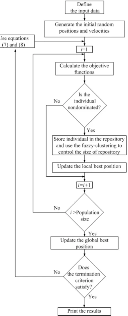
A fuzzy-based clustering procedure has been used to control

the size of the solution repository (for more details, see [19]). Figure 4 shows the MISAPSO algorithm has been used to solve the proposed multi-objective problem in Eq. (6).

3- 4- Optimum cutting parameters

To show the implementation of the proposed algorithm, the case study introduced in section 2 has been considered. The MISAPSO algorithm has been used to find optimal cutting parameters which maximize the material removal rate and minimize the surface roughness, simultaneously. Table 5

M. M. Abootorabi, AUT J. Mech. Eng., 2(1) (2018) 115-123, DOI: 10.22060/ajme.2018.12581.5373

122 shows the limitations of the input parameters.

The Monte Carlo simulation has been used to show the feasibility space of solution [22]. The main goal of the MISAPSO algorithm is to find the optimal Pareto set of the feasibility space of solution. Figure 5 shows the feasibility space of the foregoing optimization problem. The results obtained from the MISAPSO algorithm are shown in Figure 6.

The obtained results depicted in Fig. 6 show that there is no optimum solution for Eq. (6). There is a set of optimal solutions (Pareto solutions). When the surface roughness of the work piece decreases, the material removal rate decreases, as well. Some Pareto-optimal cutting parameters obtained from the MISAPSO are shown in Table 6.

When a process planner must choose a proper solution from among all others, his/her skills and experiences will help him/her to make the right choice. The proposed algorithm is able to help the process planner in selecting the optimum

cutting parameters to achieve low surface roughness and high material removal rate, simultaneously.

4- Conclusions

In the present study, using a full factorial experiment design, the effects of the cutting parameters i.e. cutting speed, feed rate, and radial depth of cut on the surface roughness in the climb milling process of stainless steel have been investigated. The main conclusions obtained from this study are as follows: 1. The feed rate was the most effective parameter on the

surface roughness. With the aid of experimental results, the multiple linear regression equation for the surface roughness has been obtained. The value of Mean Squared Error for this regression equation was 0.12 which shows a good approximation.

2. The obtained regression equation and the material removal rate (MRR) formula have been used as the objective functions in a Multi-objective Improved Self-Adaptive Particle Swarm Optimization (MISAPSO) algorithm. Consequently, the optimum cutting parameters in order to minimize the surface roughness and simultaneously maximize the MRR have been achieved.

3. In multi-objective optimization problems, a set of optimal solutions exists called the Pareto-optimal solutions. In this paper, the relatively new algorithm MISAPSO derived from PSO method has been employed to find the Pareto-optimal solutions in a cutting process and its ability for optimization has been confirmed. The performance and efficiency of MISAPSO algorithm have not yet been studied in the literature reviews of the field of machining optimization.

4. Each of the optimal points proposed by the algorithm MISAPSO corresponds to the values of three parameters cutting speed, feed rate and radial depth of cut which optimize the material removal rate and surface roughness simultaneously. In other words, for an expected amount of surface roughness, the maximum allowable material removal rate with the values of corresponding cutting parameters was recommended by this optimization algorithm.

The proposed procedure can help the process planners in selecting optimum cutting parameters in order to simultaneously reach a low surface roughness and a high

MRR.

Parameter Vmin Vmax fmin fmax ar,min ar,max

Value 15 40 0.2 0.8 0.3 0.9

Table 5. Cutting Parameters’ Limitations

Fig. 5. The feasibility space of the optimization problem

Fig. 6. The Pareto-optimal set obtained from the MISAPSO algorithm

V

(m/min) (mm/rev)f (mm)ar (µm)Ra (mmMRR3_/s)

34.4 0.31 0.86 0.94 23.9

33.5 0.32 0.84 0.95 24.2

36.2 0.49 0.90 1.36 41.4

34.5 0.54 0.84 1.38 42.3

32.4 0.59 0.88 1.44 44.5

30.0 0.71 0.87 1.61 49.4

28.8 0.76 0.86 1.68 49.9

31.7 0.74 0.90 1.69 56.0

38.8 0.79 0.88 2.11 71.4

M. M. Abootorabi, AUT J. Mech. Eng., 2(1) (2018) 115-123, DOI: 10.22060/ajme.2018.12581.5373

123 References

[1] P.G. Benardos, G.C. Vosniakos, Predicting Surface Roughness in Machining: A Review, Int J Mach Tool

Manuf, 43 (2003) 833–844.

[2] M. Chandrasekaran, M. Muralidhar, C. Murali Krishna, U.S. Dixit, Application of soft computing techniques in machining performance prediction and optimization: a literature review, Int J Adv Manuf Technol, 46 (2010) 445-464.

[3] C.X. Feng, X. Wang, Development of empirical models for surface roughness prediction in finish turning, Int J

Mach Tool Manuf, 20 (2002) 348–356.

[4] B. Ozcelik, M. Bayramoglu, The statistical modeling of surface roughness in high-speed flat end milling, Int J

Mach Tool Manuf, 46 (2006) 1395–1402.

[5] H. Aouici, M.A. Yallese, B. Fnides, K. Chaoui, T. Mabrouki, Modeling and optimization of hard turning of X38CrMoV5-1 steel with CBN tool: machining parameters effects on flank wear and surface roughness,

J Mech Sci Technol, 25 (2011) 2843–2851.

[6] S. Bharathi Raja, N. Baskar, Application of Particle Swarm Optimization technique for achieving desired milled surface roughness in minimum machining time,

Expert Syst Appl, 39 (2012) 5982–5989.

[7] T. Kivak, Optimization of surface roughness and flank wear using the Taguchi method in milling of Hadfield steel with PVD and CVD coated inserts, Measurement, 50 (2014) 19–28.

[8] G.M.A. Acayaba, P.M. Escalona, Prediction of surface roughness in low speed turning of AISI316 austenitic stainless steel, CIRP J Manuf Sci Technol, 11 (2015) 62–67.

[9] M. Hanief, M.F. Wani, Modeling and prediction of surface roughness for running-in wear using Gauss-Newton algorithm and ANN, Appl Surf Sci, 357 (2015) 1573–1577.

[10] A. Gok, A new approach to minimization of the surface roughness and cutting force via fuzzy TOPSIS, multi-objective grey design and RSA, Measurement, 70 (2015) 100–109.

[11] M. Gupta, S. Kumar, Investigation of surface roughness and MRR for turning of UD-GFRP using PCA and Taguchi method, Int J Eng Sci Technol, 18 (2015) 70-81.

[12] A. Nejat, H.R. Kaviani, Aerodynamic optimization

of a megawatt class horizontal axis wind turbine blade with particle swarm optimization algorithm, Modares Mechanical Engineering, 16(11) (2016) 1-11. (in Persian)

[13] M. Fallah, B. Moetakef Imani, Updating boring bar’s

dynamic model using particle swarm optimization,

Modares Mechanical Engineering, 16(12) (2016)

479-489. (in Persian)

[14] The Atlas Specialty Metals-Technical Handbook of

Stainless Steels, (2016). http://www.atlasmetals.com.au

[15] ISO 4287, Geometrical Product Specifications (GPS)

Surface Texture: Profile Method Terms, Definitions and Surface Texture Parameters. International Organization for Standardization, Geneva, 1997.

[16] E. Budak, A. Takeli, Maximizing Chatter Free Material Removal Rate in Milling through Optimal Selection of Axial and Radial Depth of Cut Pairs, CIRP Ann Manu Techn, 54 (2005) 353–356.

[17] M. Moradi, et al., Parameter dependencies in laser

hybrid arc welding by design of experiments and by a mass balance, Journal of Laser Applications, 26 (2014) 1-9.

[18] T. Hastie, R. Tibshirani, J. Friedman, The Elements

of Statistical Learning: Data Mining, Inference, and

Prediction, 2nd Edition, Springer-Verlag, New York,

2009.

[19] H. Zeinoddini-Meymand, B. Vahidi, R.A. Naghizadeh,

M. Moghimi, Optimal Surge Arrester Parameter Estimation Using a PSO-Based Multiobjective Approach,

IEEE Trans Power Delivery, 28 (2013) 1758-1769.

[20] R. Caponetto, L. Fortuna, S. Fazzino, M.G. Xibilia,

Chaotic sequences to improve the performance of evolutionary algorithms, IEEE Trans Evol Comput, 7 (2003) 289-304.

[21] C.M. Lin, M. Gen, Multi-criteria human resource

allocation for solving multistage combinatorial optimization problems using multi-objective hybrid genetic algorithm, Expert Syst Appl, 34 (2008) 2480-2490.

[22] N.T. Thomopoulos, Essentials of Monte Carlo

Simulation: Statistical Methods for Building Simulation

Models, Springer-Verlag, New York, 2013.

Please cite this article using:

M. M. Abootorabi, Multi-objective Optimization of Surface Roughness and Material Removal Rate Using an Improved Self-Adaptive Particle Swarm Optimization Algorithm in the Milling process, AUT J. Mech. Eng., 2(1) (2018) 115-123.