Characterization of process oriented hydrologic model behavior with temporal sensitivity analysis for flash floods in Mediterranean catchments

Hydrol. Earth Syst. Sci., 17, 2305–2322, 2013 www.hydrol-earth-syst-sci.net/17/2305/2013/ doi:10.5194/hess-17-2305-2013

© Author(s) 2013. CC Attribution 3.0 License.

EGU Journal Logos (RGB)

Advances in

Geosciences

Open Access

Natural Hazards

and Earth System

Sciences

Open Access

Annales

Geophysicae

Open Access

Nonlinear Processes

in Geophysics

Open Access

Atmospheric

Chemistry

and Physics

Open Access

Atmospheric

Chemistry

and Physics

Open Access

Discussions

Atmospheric

Measurement

Techniques

Open Access

Atmospheric

Measurement

Techniques

Open Access

Discussions

Biogeosciences

Open Access Open Access

Biogeosciences

Climate

of the Past

Open Access Open Access

Climate

of the Past

Discussions

Earth System

Dynamics

Open Access Open Access

Earth System

Dynamics

Discussions

Geoscientific

Instrumentation

Methods and

Data Systems

Open Access

_{Geoscientific}

Instrumentation

Methods and

Data Systems

Open Access

Discussions

Geoscientific

Model Development

Open Access Open Access

Geoscientific

Model Development

Discussions

Hydrology and

Earth System

Sciences

Open Access

Hydrology and

Earth System

Sciences

Open Access

Discussions

Ocean Science

Open Access Open Access

Ocean Science

Discussions

Solid Earth

Open Access Open Access

Solid Earth

Discussions

The Cryosphere

Open Access Open Access

The Cryosphere

Discussions

Natural Hazards

and Earth System

Sciences

Open Access

Discussions

Characterization of process-oriented hydrologic model behavior

with temporal sensitivity analysis for flash floods in Mediterranean

catchments

P. A. Garambois1,2, H. Roux1,2, K. Larnier1,2, W. Castaings3, and D. Dartus1,2

1_{Universit´e de Toulouse, INPT, UPS, IMFT (Institut de M´ecanique des Fluides de Toulouse), All´ee Camille Soula,}

31400 Toulouse, France

2_{CNRS, IMFT, 31400 Toulouse, France}

3_{EDYTEM, Universit´e de Savoie, Le Bourget du Lac cedex, France} Correspondence to: P. A. Garambois ([email protected])

Received: 4 December 2012 – Published in Hydrol. Earth Syst. Sci. Discuss.: 28 January 2013 Revised: 21 May 2013 – Accepted: 21 May 2013 – Published: 27 June 2013

Abstract. This paper presents a detailed analysis of 10 flash

flood events in the Mediterranean region using the distributed hydrological model MARINE. Characterizing catchment re-sponse during flash flood events may provide new and valu-able insight into the dynamics involved for extreme catch-ment response and their dependency on physiographic prop-erties and flood severity. The main objective of this study is to analyze flash-flood-dedicated hydrologic model sensi-tivity with a new approach in hydrology, allowing model outputs variance decomposition for temporal patterns of pa-rameter sensitivity analysis. Such approaches enable rank-ing of uncertainty sources for nonlinear and nonmonotonic mappings with a low computational cost. Hydrologic model and sensitivity analysis are used as learning tools on a large flash flood dataset. With Nash performances above 0.73 on average for this extended set of 10 validation events, the five sensitive parameters of MARINE process-oriented dis-tributed model are analyzed. This contribution shows that soil depth explains more than 80 % of model output variance when most hydrographs are peaking. Moreover, the lateral subsurface transfer is responsible for 80 % of model vari-ance for some catchment-flood events’ hydrographs during slow-declining limbs. The unexplained variance of model output representing interactions between parameters reveals to be very low during modeled flood peaks and informs that model-parsimonious parameterization is appropriate to tackle the problem of flash floods. Interactions observed af-ter model initialization or rainfall intensity peaks incite to

improve water partition representation between flow com-ponents and initialization itself. This paper gives a practi-cal framework for application of this method to other mod-els, landscapes and climatic conditions, potentially helping to improve processes understanding and representation.

1 Problem framework

1.1 Flash flood modeling complexity

The Mediterranean climatic zone is prone to heavy rain-fall events especially during the rain-fall season. Either quasi-stationary mesoscale convective systems, which can last sev-eral hours, or frontal disturbances blocked by the mountains can produce high precipitation totals (Nuissier et al., 2008) that trigger severe flash floods. The high variability of pre-cipitations (Moussa et al., 2007) along with topography in-fluence and spatial distribution of soil and land use proper-ties makes hydrological processes largely variable both in time and space (Pilgrim et al., 1988). Flash floods are ex-treme catchment responses with high peak discharge often produced by severe localized thunderstorms. They are one of the most destructive hazards in the Mediterranean region and have caused casualties and billions of euros of damages in France over the last two decades (Gaume et al., 2009).

These events often reveal aspects of hydrological behav-ior that either were unexpected on the basis of weaker re-sponses or highlight anticipated but previously unobserved

behavior (Delrieu et al., 2005). Characterizing the response of a catchment during flash flood events thus may provide new and valuable insight into processes for extreme flood response and their dependency on catchment properties and flood severity (Borga et al., 2008).

In the literature, several approaches are proposed for flash flood events modeling and/or prediction, each with its speci-ficities depending on perception and parameterization of the dominant hydrological processes (Moussa et al., 2007; Saulnier and le Lay, 2009; Braud et al., 2010; Roux et al., 2011) among others for the Mediterranean region. These models often take advantage of available data in order to as-sign spatially distributed forcing as well as distributed catch-ment parameters. However, increasing model complexity can lead to overparameterization and equifinality problems be-cause of high dimensionality and multi-modal response sur-face. As a result, parameter values might not be identifiable in the calibration process (Beven, 1989). Sieber and Uhlen-brook (2005) have highlighted that sensitivity analysis (SA) can not only identify the most important parameters but also contribute to understanding and improving the structure of hydrologic model.

1.2 Understanding uncertainty with sensitivity analysis

Sensitivity analysis (SA) assesses the impact of model pa-rameters on the output, and is therefore a convenient tool to investigate model behavior and especially the importance of particular parameterizations within the model. SA has be-come a popular tool in catchment modeling to explore high dimensional parameter spaces, assess parameter identifiabil-ity, and understand sources of uncertainty (Hornberger and Spear, 1981; Freer et al., 1996; Wagener et al., 2001; Hall et al., 2005; van Griensven et al., 2006; Tang et al., 2007). Some studies highlight the usefulness of sensitivity analysis for the improvement of hydrological models (Andr´eassian et al., 2001; Oudin et al., 2006; Castaings et al., 2007; Ratto et al., 2007b; Tang et al., 2007; Pushpalatha et al., 2011). Other studies used SA to better understand model behavior with re-spect to inputs such as precipitation (Xu et al., 2006; Meselhe et al., 2009).

With the current shift toward model complexification and/or real-time hydrometeorological forecasts, of prior im-portance is the understanding of uncertainty and its sources. In catchment modeling it can be achieved with various meth-ods, of which formal Bayesian methods (Kuczera and Parent, 1998) and the GLUE method (Beven and Binley, 1992) are the most popular, as well as recursive application of RSA for dynamic identifiability analysis (Wagener et al., 2003) or Bayesian total error analysis (BATEA) method (Kavet-ski et al., 2006) for comprehensive calibration and uncer-tainty estimation. According to Saltelli et al. (2004) sensi-tivity analysis is the study of how uncertainty in the output of a model can be apportioned to different sources of uncer-tainty in the model input. Sensitivity analysis is recognized

as a helpful parameter-space screening tool to identify key parameters controlling the performances. It can help in re-ducing problem dimensionality with factor fixing (FF) for noninfluential parameters, and factor prioritization (FP) for those controlling the most model output uncertainty (Saltelli et al., 2000). Besides the selection of the appropriate method for analyzing parameter sensitivity depends strongly on the goal of the sensitivity analysis (Saltelli et al., 2006). Of par-ticular interest is the analysis of the dependence of the model output variance to simultaneously modified parameters; this can be achieved with methods based on variance decomposi-tion (Efron and Stein, 1981; Sobol, 1993). The applicadecomposi-tion of three sensitivity analysis methods including Sobol’s method by Massmann and Holzmann (2012) shows that the two most important parameters of their conceptual continuous rainfall– runoff model are correctly identified as being sensitive by all methods.

1.3 Variance-based methods and temporal sensitivity analysis

Variance-based methods result in reliable estimates of sensi-tivities even for nonlinear and nonmonotonic models, as was often demonstrated using examples where analytical solu-tions can be calculated (Saltelli and Bolado, 1998). The price to be paid in order to relax all assumptions on model behavior is that the required number of model runs is relatively high (>1000) for most approaches. Some variants of this method, in terms of partial variances calculation, are Sobol’s method (Sobol, 1990, 2001) and the extended Fourier amplitude sen-sitivity test ((E)FAST) (Cukier et al., 1973; Saltelli and Bo-lado, 1998; Fang et al., 2003; Reusser et al., 2011).

Variance-based sensitivity analysis methods aim to quan-tify the amount of variance that each parameter contributes to the unconditional variance of the model output. These amounts are characterized by first order or interaction effects expressed as sensitivity indices (Si’s). Despite its high

com-putational demands contributions (Saltelli, 2002) and try-ing to make it more effective, the powerful Sobol SA tech-nique, for example, has recently become more popular in en-vironmental modeling (Pappenberger et al., 2007, 2008; Van Werkhoven et al., 2008; Jing, 2011; Li et al., 2012).

Tang et al. (2007) compared state of the art in sensitiv-ity analysis including Sobol’s method and found it to be the most effective in estimating first-order parametric sensitivi-ties and overall influence including interaction effects. Tang et al. (2007) make a step-wise analysis of a conceptual grid-base-distributed rainfall–runoff model (HL-RDHM). Their sensitivity analysis reveals the impact of rainfall distribution on spatial sensitivities and input variables mostly controlling HL-RDHM’s behavior. The use of Sobol indices for sensitiv-ity analysis purposes is investigated by Nossent et al. (2011) in the case of a SWAT model. They conclude that in general the Sobol sensitivity analysis can be successfully applied for factor fixing and factor prioritization with respect to the input

parameters of a SWAT model, even with a limited number of model evaluations. The analysis also supports the identifi-cation of model processes, parameter values and parameter interaction effects. Some of the recent studies applying SA to rainfall–runoff, flood inundation, and water quality mod-els are listed by Reusser et al. (2011); 8 out of the 18 studies use variance-based methods. In seven studies, on the order of 10 000 model runs were computed to calculate sensitivities, which is impossible for computationally expensive models. As highlighted by Reusser et al. (2011), analyzing tempo-ral dynamics of parameter sensitivity (TEDPAS) of model output variables, such as discharge, we can quantify which model components dominate the simulation response. Their analysis reveals that temporal dynamics of model parame-ter sensitivity can be a powerful tool for hydrological model analysis, especially to identify parameter interaction as well as the dominant hydrological response modes. Reusser and Zehe (2011) with TEDPAS (temporal dynamics of parameter sensitivity) and TIGER (time series of grouped error) meth-ods investigate parameter uncertainty for perimeth-ods of poor model efficiencies. With modeling and temporal sensitivity analysis used as learning tools, WaSIM-ETH complex grid-based model hypotheses are shown to be insufficient to de-scribe Weisseritz headwater catchment behavior and future developments seem required.

1.4 Scope of the paper

The core idea of this paper is to approach hydrologic model sensitivity with temporal sensitivity analysis, here in the case of quick and strong catchment flash flood responses. The originality lies in TEDPAS analysis calculated from variance-based decomposition that may reveal sensitivity peaks and thus flow dynamics at key instants. This kind of analysis is new for hydrologic models especially for event-process-oriented distributed models. Using TEDPAS as a di-agnostic tool joins the idea of dynamic identifiability intro-duced by Wagener et al. (2003). But these two methods serve a different purpose since it is a necessary but insufficient con-dition that parameters must be sensitive in order to be identi-fiable whereas sensitive parameters may not be identiidenti-fiable.

In this contribution, a temporal sensitivity analysis of the process-oriented spatially distributed MARINE model dedi-cated to flash floods is carried out. Based on the understand-ing of Mediterranean catchments hydrological processes the hydrological rainfall–runoff model MARINE (Mod´elisation et Anticipation du Ruissellement et des Inondations pour des ´ev`eNements Extrˆemes) aims at (i) exploiting the potential of distributed models (ii) using physically meaningful parame-ters, while (iii) maintaining a simple and parsimonious pa-rameterization (Roux et al., 2011). Given a validated model structure for flash floods in the French Mediterranean region, the question of sensitivity is approached in a probabilistic framework. One parameter set for each of the six catchments is tested on validations events for which the analysis of

TED-PAS is performed. The procedure is implemented for con-trasted hydrometeorological events in the C´evennes and the Pyrenean region (France) with the view to bring understand-ing in model behavior for contrasted catchments and flash flood events on steep terrains and complex geo-pedological formations.

The paper is organized as follows. Section 2 describes variance decomposition method and sensitivity indices cal-culation. MARINE model and the six Mediterranean catch-ments of interest are presented in Sect. 3. Catchment param-eter sets and their efficiencies on 10 validation events are calculated and temporal sensitivity analysis hypotheses are tested in Sect. 4. Then TEDPAS on these validation events are examined in Sect. 5. After a conclusion on the results, processes, variables and parameters that require further de-scription or observations are emphasized and the possibility of applying this method to improve the understanding of the major processes involved in flood events is discussed.

2 Background on model analysis with variance decomposition methods

Thoughtful descriptions of sensitivity analysis methods can be found in Saltelli et al. (2000). Variance-based meth-ods are part of the practices Saltelli and Annoni (2010) recommended as an alternative to OAT analysis (one at a time method: local analysis evaluating separately the effect of each individual parameter). Variance-based methods are based on a decomposition of the model output variance.

Letk∈ <k denote the set of all possible values that the

model parameters can assume. Let X∈k be a possible

value of thek model parameters normalized by their varia-tion range. We denote byY=g(X)=g(X1, . . ., Xk)the

re-lationship that links the model inputs to the model output. The parameters X have a domain of validity linked to the uncertainty about their precise value.

Assuming thatgis a square integrable function overk=

{_X|0≤Xi ≤1;i=1, . . ., k}, it can be decomposed using an

expansion with summand gi...p (X1, . . ., Xp)of increasing

dimensionalityp < k:

Y =g(X)=g0+ k

X

i=1

gi(Xi)+ k

X

i=1

X

i>j

gij(Xi, Xj)

+. . .+g1,2,...,k(X1, X2, . . ., Xk). (1)

Sobol (1993) proved that this HDMR decomposition (high-dimension model representation) was unique if each term in the expansion has zero mean, then all the terms of the de-composition are orthogonal in pairs:

Z

k

gi1,...,ipgi1,...,isdX=0. (2)

The total unconditional variance of model output can be de-fined as

V (Y )=

Z

k

g2(X)dX−g₀2. (3)

The partial variances which are the components of the to-tal variance decomposition are computed from each term in Eq. (1) as

Vi,...,p= 1

Z

0 1

Z

0

g_i2

1,...,ip(Xi1, . . ., Xip)dXi1, . . .,dXip. (4)

The relation (3) expressed with Eqs. (1) and (4) leads to the so-called functional ANOVA decomposition:

V (Y )=X

i

Vi+

X

i

X

j >i

Vij+. . .+V1,2,...,k, (5)

whereV (Y ) is the total variance,Vi is the variance caused

by parameterXi (first-order variance),Vij is the covariance

caused byXiandXj (second-order variance), and higher

or-der terms show the variance contribution from multiple pa-rameters. The two factorsXiandXjare said to interact when

their effect onY cannot be expressed as the sum of their sin-gle effectsVi andVj. Interactions may imply, for instance,

that extreme values of the model output are uniquely associ-ated with particular combinations of model inputs in a way that is not described by first-order effectsSi.

From this relation (5), sensitivity indices can be defined in order to assess the sensitivity ofY toX when X is un-certain. The first-order effect representing the average output variance reduction that can be achieved whenXi is fixed is

defined by

Si=

Vi

V =

V (Y )−EXi[V (Y|Xi)]

V (Y ) =

VXi[E (Y|Xi)]

V (Y ) . (6) The partial varianceVi in Eq. (6) is given by the variance of

the conditional expectationVi=VXi[E (Y|Xi)] and is also

called the main effect ofXi onY. The impact on the model

output variance of the interactions between parameters Xi

andXjis given bySij=Vij/V and it can be generalized in

interactions effects up to orderkby replacing the indexiby the corresponding set of input factors.

The estimation of partial variances could be very expen-sive with brute-force methods, but a shortcut was proposed by Sobol to reduce the calculation of the double-loop inte-grals of Eq. (4). Efficient methods such as extended FAST from Saltelli (1999) or improved Sobol from Saltelli (2002) were proposed in order to estimate bothSiandST ifor all

in-puts factors for a computational cost ofN (k+2). However, alternatives techniques were introduced recently, allowing the estimation ofS_i0sand low interaction effects (up to order 3) for a computational cost independent fromk(i.e., equal to

N the sample size) (RBD-FAST from Tarantola et al., 2006; Mara, 2009; Storlie and Helton, 2007; Oakley and O’Hagan, 2004; Sudret, 2008; Crestaux et al., 2009).

The method used in this paper is the state-dependent pa-rameter (SDP) metamodeling method (Ratto et al., 2007a) which is based on recursive filtering and smoothing estima-tion to build an approximaestima-tion of the computaestima-tional model. Ideas and tools from signal processing and time series analy-sis are used to estimate the terms in the ANOVA-HDMR de-composition using a special recursive fixed-interval smooth-ing algorithm that estimates the parameters in an SDP for-mulation of the input–output mapping (Ratto et al., 2007a). It is a very efficient method that does not require any spe-cific rule for sampling inputs, and provides fastly accurate and unbiaised results for both sensitive and insensitive in-puts according to (Gatelli et al., 2009). Ratto et al. (2007a) show that even for a large number of parameters the SDP method allows a good estimation of variance-based sensi-tivity indices with a mild computational cost for models with up to 20 input factors. In the following we use the routine SS-ANOVA (available at http://sensitivity-analysis. jrc.ec.europa.eu/software/index.htm). The recursive filtering and smoothing procedure provides standard errors of the esti-mated state-dependant parameters and hence the relative sig-nificance of estimated HDMR terms and sensitivity indices.

3 Model and site description

3.1 MARINE flash flood model

The modeling approach is the distributed model MARINE for flash flood forecasting (Roux et al., 2011) with a sub-surface transfer module. The predominant factor determin-ing the formation of runoff is represented by the topogra-phy: slope and downhill directions. MARINE runs on a fixed time step and is structured into three main modules (Fig. 1). The first module allows separating the precipitation into sur-face runoff and infiltration using the Green and Ampt model; the second module represents subsurface downhill flow with an approximation of the Darcy’s law and the standard TOP-MODEL transmissivity profile (Beven and Kirkby, 1979) and the third one the overland flow (over hillslopes and in the drainage network): the transfer function component al-lows routing the rainfall excess to the catchment outlet us-ing the kinematic wave approximation. Both infiltration ex-cess and saturation exex-cess are represented within MARINE. The spatial discretization of the catchment is performed us-ing the digital elevation model grid resolution, a regular grid of squared cells. Evapotranspiration is not represented since the model purpose was to simulate individual flood events during which such process is negligible. Cell soil moisture deficit is initialized from a continuously distributed water balance model output briefly described later. For a complete

38 1

2

Figure 1: MARINE model structure, parameters and variables. Green and Ampt 3

infiltration equation: infiltration rate i (m.s−1), cumulative infiltration I (mm), saturated 4

hydraulic conductivity K (m.s−1), soil suction at wetting front ψ (m), saturated and initial 5

water contents are respectively θs and θi (m3 m−3). Subsurface flow: local transmissivity of

6

fully saturated soil T0 (m2s−1), saturated and local water contents are θs and θ (m3 m−3),

7

transmissivity decay parameter is m (–), local slope angle β (rad). Kinematic wave: water 8

depth h (m), time t (s), overland flow velocity u (m.s−1_{), space variable x (m), rainfall rate} 9

r (m.s−1_{), infiltration rate i (m.s}−1_{), bed slope S (m.m}−1_{), Manning roughness coefficient n} 10

(m−1/3_.s). 11

12 13

Fig. 1. MARINE model structure, parameters and variables. Green and Ampt infiltration equation: infiltration ratei(m s−1), cumula-tive infiltrationI(mm), saturated hydraulic conductivityK(m s−1), soil suction at wetting frontψ(m), saturated and initial water con-tents are respectivelyθs andθi (m3m−3). Subsurface flow: local transmissivity of fully saturated soilT0(m2s−1), saturated and lo-cal water contents areθsandθ(m3m−3), transmissivity decay pa-rameter is m (–), local slope angleβ(rad). Kinematic wave: water depthh(m), timet(s), overland flow velocityu(m s−1), space vari-ablex(m), rainfall rater (m s−1), infiltration ratei(m s−1), bed slopeS(m m−1), Manning roughness coefficientn(m−1/3s−1).

description of the MARINE model the reader can refer to Roux et al. (2011).

3.2 Study zone

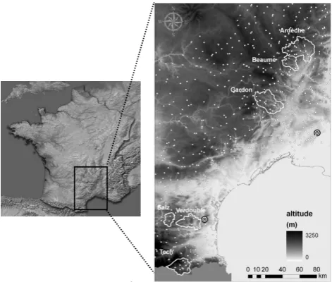
The proximity of the Mediterranean Sea and the steep sur-rounding orography can promote low-level flow lifting in an unstable atmosphere, as for the Alps and Pyrenees (Davolio et al., 2009; Tarolli et al., 2012). The highest flooding risk is in autumn with wet soils and maximum rainfall rates. Sum-mers are hot and dry; however summer storms also represent a nonnegligible flooding risk. The density of both hydrom-eteorological radar and hourly rain gauge coverage offers interesting possibilities for flood-triggering rainfall monitor-ing and quantitative precipitation estimation (Fig. 2). Thus the French Mediterranean region rather frequently affected by intense rainfalls represents an interesting area for flash flood study in a regional manner (Garambois et al., 2012b) with contrasted catchment properties, rainfall distributions and hydrological response characteristics (Garambois et al., 2012a).

From the Pyrenean foothills and the Corbi`eres Mountains in the south to the C´evennes foothills and the Ard`eche region, six flood-prone catchments with areas ranging from 144 to 619 km2and contrasted physiographic properties are selected (Table 1). They present a highly marked topography with nar-row valleys and steep hillslopes (Fig. 2). A DEM data file of the study site with a grid scale of 25 m was available from the National Geographic Institute (BD TOPO®©IGN – Paris –

39 1

2

Figure 2: (Left) France topography (source: SRTM image, NASA/JPL). (Right) (white 3

contour) Topography of the six catchments of interest (France), BD TOPO® IGN, 4

(concentric circles) Hydrometeorological radars, (white dots) operational raingauges. 5

6

Fig. 2. (Left) Topography of France (source: SRTM image, NASA/JPL). (Right) (white contour) Topography of the six catch-ments of interest (France) from BD TOPO® IGN, (concentric circles) hydrometeorological radars, (white dots) operational rain gauges.

2008.©(SCHAPI)). The mean elevation ratios of the whole

river basins are above 0.025 m m−1.

The Salz and Verdouble catchment areas mainly develop on sedimentary formations contrarily to the other catch-ments, where substrates develop on metamorphic and plu-tonic terrains. Soil thicknesses and textures were available from the BDSol-LR (Robbez-Masson et al., 2002) (IGCS – BDSol-LR – version no. 2006, INRA – Montpellier SupA-gro) (Table 1). Soil-saturated hydraulic conductivities, satu-rated water contents and soil suctions are determined with (Rawls and Brakensiek, 1985) pedotransfer functions as pro-posed by Manus et al. (2009). Braud et al. (2010) and Roux et al. (2011) highlight the importance of soil thickness and tex-ture on hydrological process and catchment flood response. It has recently been shown with a comparative hydrologic study that flood response in Austria is significantly controlled by geology (Ga´al et al., 2012).

For the Gardon, Beaume and Ard`eche catchments, vege-tation is dense and mainly composed of chestnut trees, pas-ture, holm oaks, conifers, waste land and garrigue. Chest-nut trees are located in the upstream area and on the south-facing slopes (sunny sides or adret), while forested garrigues and holm oaks are located in the downstream area and on the north-facing slopes (shady sides or ubac). The Tech catchment’s vegetation is rather dense also, with broadleaved and coniferous forests. Mainly Mediterranean forest, garrigue, holm oaks and vineyards are encountered on the Salz and Verdouble catchments. A vegetation and land use map (Corine Land Cover provided by the Service de l’Observation et des Statistiques (SOeS) of the French

Table 1. Catchments physiographic properties, elevation ration is height difference divided by longest flow path length, K mean is the mean soil saturated hydraulic conductivity. Hsol is the spatially distributed soil depth estimated from pedologic data.

Max.

Height flow Elevation Hsol Hsol Hsol Hsol Soil K

Area diff. length ratio min. max. mean std volume mean Catchments (km2) (m) (km) (m m−1) (m) (m) (m) (m) (m3) (mm h−1) Tech (Pas-du-Loup) 250 2730 34.5 0.079 0.00 0.69 0.16 0.13 5.3×107 2.5 Verdouble (Tautavel) 299 915 37.0 0.025 0.08 0.63 0.33 0.16 1.0×108 2.4 Salz (Cassaignes) 144 995 17.2 0.058 0.00 0.74 0.31 0.19 4.2×107 3.9 Gardon (Anduze) 543 1065 45.1 0.024 0.08 0.64 0.28 0.12 1.5×108 05.0 Beaume (Rosi`eres) 212 1360 29.0 0.047 0.05 0.49 0.25 0.07 5.2×104 8.7 Ard`eche (Vog¨u´e) 619 1380 52.5 0.026 0.05 0.50 0.28 0.08 1.7×108 8.7

40

0 1 2 3 4 5 6 7

0 1 2 3 4 5 6 7

Qpspe obs (m3/s/km2)

Qpspe sim (m

3/s/km 2)

1

2

Figure 3: Simulated peak discharge versus observed peak discharge for validation events

3

with first bisector (blue line).

4

Fig. 3. Simulated peak discharge versus observed peak discharge for validation events with first bisector (blue line).

Ministry of Environment, www.ifen.fr) is used to derive distributed surface roughness.

4 Preliminary analysis

Initialization is an important step in the case of flash flood event-based models running on a time window of few days. Soil saturation at the beginning of each event is estimated with SAFRAN-ISBA-MODCOU (SIM), a continuous hy-drometeorological model (Habets et al., 2008). This contin-uous water balance model is run over the whole country on 8 km×8 km cells and outputs such as soil moisture with at least daily time step are available. This systematically avail-able spatial–temporal model outputs for catchment initial soil moisture accountancy is chosen. We keep in mind that soil moisture is related to soil parameters in defining catch-ment soil infiltrability and storage capacity. But an accurate estimation of soil moisture at the catchment scale is still difficult even if combining spatialized superficial remotely

41

Time (h)

O

b

se

rve

d

d

is

ch

ar

ge

s (

m

3/s

)

R

ai

n

fal

l i

n

te

n

si

ty (

m

m

/h

)

0 5 10 15 20 25 30 35

0 1000 2000 3000 4000

0

20

40

60

80

100 08_09_2002

Rainfall intensity (mm/h) Q10 of simulated discharges Q90 of simulated discharges

Time (h)

F

ir

st

or

d

er

s

en

si

ti

vi

ty

0 5 10 15 20 25 30 35

0 0.2 0.4 0.6 0.8 1

Si1_CZ 5 % Si1_CZ10 % Si1_CZ15 %

1 2

Figure 4: (Top) Gardon d’Anduze 08/09/2002 flash flood event and quintiles Q10 and Q90

3

of simulated discharges for α = 5, 10 and 15 %. (Bottom) First order effects for CZ and

4

three sampling ranges. 5

6

Fig. 4. (Top) Gardon d’Anduze: 8 September 2002 flash flood event and quintilesQ₁₀ andQ₉₀ of simulated discharges forα=5, 10 and 15 %. (Bottom) First-order effects forCZ and three sampling ranges.

sensed data and numerous in situ point measurements lead to promising results (Brocca et al., 2012; Albergel et al., 2012). An estimation of uncertainty for soil moisture model outputs would be welcome but it remains a hard task given that a very good knowledge of soil properties and structure seems to be required.

4.1 Calibrated parameter sets

In order to avoid a model overparameterization, spatial pat-terns of several parameters are derived from soil surveys, and a unique correction coefficient is then applied to each param-eter map. This approach has been chosen for three parame-ters – namely the distributed saturated hydraulic conductivity K, the lateral transmissivityT0and soil thicknessesZ. The

calibration procedure consists in estimating the following:

42 Time (h)

O

b

se

rv

ed

d

is

ch

a

rg

es

(

m

3/s

)

R

a

in

fa

ll

i

n

te

n

si

ty

(

m

m

/h

)

0 50 100 150 200 250

0 500 1000

1500 0

20 40 60 80 100

QObs 3evs Vogüé Rainfall (mm/h) Q10

Sim

Q90 Sim

Time (h)

F

ir

st

o

rd

er

s

en

si

ti

v

it

y

0 50 100 150 200 250

0 0.2 0.4 0.6 0.8 1

CKss

KD2

KD1

C_k CZ

1

2

Figure 5: (Top) Ardèche at Vogüé (619 km²), 20/10/2008, 31/10/2008 and 03/11/2011 3

flash flood events and quintiles Q10 and Q90 of simulated discharge. (Bottom) first order

4

effects representing first order contribution, partial variances out of model output variance 5

(-). 6

Fig. 5. (Top) Ard`eche at Vog¨u´e (619 km2): 20 October 2008, 31 October 2008 and 3 November 2011 flash flood events and quintilesQ10 andQ90of simulated discharge. (Bottom) First-order effects representing first-order contribution and partial variances out of model output variance (–).

43 Time (h)

O

b

se

rv

ed

d

is

ch

a

rg

es

(

m

3/s

)

R

a

in

fa

ll

i

n

te

n

si

ty

(

m

m

/h

)

0 20 40 60 80 100 120

0 1000 2000 3000 4000

5000 0

20 40 60 80 100

QObs 3evs Gardon Rainfall (mm/h) Q10

Sim

Q90 Sim

Time (h)

F

ir

st

o

rd

er

s

en

si

ti

v

it

y

0 20 40 60 80 100 120

0 0.2 0.4 0.6 0.8 1

CKss

KD2

KD1

Ck

C_Z

1

2

Figure 6: (Top) Gardon at Anduze (543 km²), 28/09/2000, 08/09/2002 and 18/10/2006 3

flash flood events and quintiles Q10 and Q90 of simulated discharge. (Bottom) first order

4

effects. 5

6

Fig. 6. (Top) Gardon at Anduze (543 km2): 28 September 2000, 8 September 2002 and 18 October 2006 flash flood events and quintilesQ10 andQ90of simulated discharge. (Bottom) First-order effects.

three coefficients of correction for spatialized data; one for the saturated hydraulic conductivities, namedCK; another

one,CKSS, for the lateral subsurface flow transmissivity (T0);

and the last one for the soil thicknesses, named CZ, the

Strickler roughness of the main channelKD1and the

Strick-ler roughness of the overbank of the drainage networkKD2

(Roux et al., 2011; Garambois et al., 2012a). Concerning the transmissivityT0the spatial variability is taken from the

hy-draulic conductivity map. Catchment parameter sets that will be used in this paper are given in Table 2. For each catch-ment, model calibration is performed by estimating a param-eter set over several flash flood events (Table 3); that is, a cost function equal to 1-Nash is minimized over multiple flood

events (called global Nash hereafter). The minimization tech-nique is a BFGS (Broyden–Fletcher–Goldfarb–Shanno) al-gorithm considering multiple starting points in the parameter space. The validation is performed on other available flash flood events, and efficiencies are given in Table 3. We do not pretend to have reached “the best parameter sets” for these catchments, the word optimal needing to be defined in func-tion of the modeling goals, especially if modeling (and data) uncertainties and parameter values are considered variable in time. Nevertheless, performances of the model on the events considered in calibration and in validation are rather high over the six catchments of interest (Table 3). Performance de-crease is slight for the whole catchment set from calibration

to validation with mean Nash values of 0.86 and 0.7, respec-tively (Table 3).

4.2 Selected validation flash flood events for sensitivity analysis

Monitoring flash floods remains a hard exercise (Borga et al., 2008) since conventional measurement networks of rain and river discharges are not able to sample effectively be-cause of scales problems. Hydrometric data are provided by the SCHAPI (Service Central Hydrom´et´eorologique d’Appui `a la Pr´evision des Inondations – French central flood fore-cast center) and the SPC Grand Delta located in Nˆımes and the SPC Mediterran´ee Ouest located in Carcassone (Service de Pr´evision des Crues – Regional flood forecast center). Radar rainfall measurements (M´et´eo France – Nˆımes radar) combined with rain gauge data are available at 5 min time steps and 1 km×1 km spatial resolution since 2002 for the whole French Mediterranean region and since 1994 on the C´evennes region. Few floods of several years return period have been experienced in the six catchments of interest catch-ment since 2002 (resp. 1994). In this paper an interesting set of 10 validation events is used. This constitutes a large val-idation dataset given the scarcity of data about flash flood events in general.

Validation event hydrographs with distinct shapes rep-resent contrasted hydrological responses to different res-onances between rainfall spatio-temporal distribution and catchment physiographic properties, in other words a catch-ment’s spatial and temporal dampening effect (cf. Table 4 and Figs. 5 to 8):

– single-peak medium events (15 March 2011 at

Pas-du-Loup, 20 December 2000 at Cassaignes, 28 Septem-ber 2000 and 18 OctoSeptem-ber 2006 with a slow-rising limb at Anduze),

– singlepeak medium events with slowrising and/or

-declining limb (16 November 2006 at Rosi`eres, 20 Oc-tober 2008 and 31 OcOc-tober 2008 at Vog¨u´e),

– multipeak events (15 March 2011 at Tautavel, 3

Novem-ber 2011 at Vog¨u´e),

– and a 50 yr return period extreme event (8

Septem-ber 2002 at Anduze).

In addition to classical normalized least-squares criterion, LNP (Table 5) considers features characterizing the flood

peak (discharge value and time to peak) (Roux et al., 2011). Efficiencies for these validation events considered in the fol-lowing are high, withLNPefficiencies above 0.73 and of 0.83

on average. Mean peak flow discharge and timing relative er-rors are inferior to 0.17 and 0.13.

Most validation events present observed specific peak dis-charge ranging from 1.13 to 2.69 m3s−1km−2(Fig. 3). The extreme event of September 2002 at Anduze has an estimated

peak discharge of 6.08 m3s−1_km−2_{. Differences between}

simulated and observed discharges are satisfactory with an R2 of 0.87 with respect to the first bisector, so the model presents no significant bias for these catchments floods.

Performances of the model on the events considered in cal-ibration and in validation are rather high over the six catch-ments of interest and may therefore be considered as suffi-cient for flash flood prediction purpose. Yet we would like to point out that the aim of this paper is not to test the predictive performances of the model, which would require a larger set of events under various conditions.

4.3 Evaluation of temporal sensitivity analysis method

Using the variance-based sensitivity analysis method de-scribed in Sect. 2, a region of the parameter space around calibration point is explored and sensitivity indices are es-timated in order to analyze the relative importance of MA-RINE model inputs for validation events. Concerning the locality (in the parameter space) of the proposed analysis, global sensitivity analysis of MARINE model has already been tested (Roux et al., 2011). The present paper investi-gates the other types of information that a temporal sensi-tivity analysis can provide. The answer to the question of how sensitivities change for different parameter sets is not straightforward, and further studies would be welcome – for example with several parameter sets for one catchment.

For each catchment we use the calibrated parameter sets of Section 4.1 for validation events and temporal parame-ter sensitivity (S_i0s)calculation. The tested input factors are the five calibrated ones: three coefficients of correctionCK,

CKss, CZ, the Strickler roughness of the overbank of the

drainage networkKD2and the main channel roughness

co-efficientKD1.

We use a 1024-parameter-set quasi-random Monte Carlo sample. The S_i0s are calculated for MARINE discharge at each time step in a±α% interval around the nominal pa-rameter value with the method described in section above. Ideally for each parameter, the sampling range around nom-inal parameter value could be defined with information on parameter posterior distribution function with the strength of methods such as Markov chain Monte Carlo (Smith and Mar-shall, 2008; Vrugt et al., 2009; Kuczera et al., 2010). These methods are, however, too computationally demanding for our extended study and the choice ofαis tested here.

From 5 to 15 % around the nominal parameter values, the choice ofαreveals to have a rather limited influence on tem-poral dynamics of parameter sensitivity (TEDPAS) and their values (Table 6). The first-order effectSi1measures the

rel-ative importance of an individual input variableXi in

driv-ing the uncertainty. Parameter rankdriv-ing remains the same with a total standard error lower than 0.03. Low error and high first-order metamodelR2attest the good convergence of the SDR algorithm on the 1024 sample size.Si values

quanti-fying model output sensitivity to each parameter are quite

Table 2. Catchment parameter sets and Nash efficiencies for multiple events calibration.

Area Global

Catchments (km2) CZ CK CKSS KD1 KD2 Nash Tech (Pas-du-Loup) 250 4.34 11.0 1515 4.83 3.24 0.90 Verdouble (Tautavel) 299 1.30 15.0 4486 5.00 3.99 0.88 Salz (Cassaignes) 144 0.95 20.0 5595 5.00 2.54 0.89 Gardon (Anduze) 543 4.60 10.3 4540 11.70 9.70 0.88 Beaume (at Rosi`eres) 212 5.30 7.40 3712 21.40 14.70 0.80 Ard`eche (at Vog¨u´e) 619 3.40 2.10 4891 10.00 19.10 0.80 Calibration ranges 0.1–10 0.1–15 100–10 000 4–40 2–30

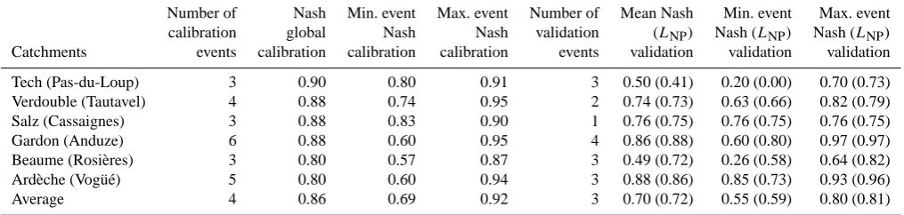
Table 3. Number of events used for calibration and validation, event and global model efficiencies of parameter sets presented in Table 2.

Number of Nash Min. event Max. event Number of Mean Nash Min. event Max. event calibration global Nash Nash validation (LNP) Nash (LNP) Nash (LNP) Catchments events calibration calibration calibration events validation validation validation

Tech (Pas-du-Loup) 3 0.90 0.80 0.91 3 0.50 (0.41) 0.20 (0.00) 0.70 (0.73) Verdouble (Tautavel) 4 0.88 0.74 0.95 2 0.74 (0.73) 0.63 (0.66) 0.82 (0.79) Salz (Cassaignes) 3 0.88 0.83 0.90 1 0.76 (0.75) 0.76 (0.75) 0.76 (0.75) Gardon (Anduze) 6 0.88 0.60 0.95 4 0.86 (0.88) 0.60 (0.80) 0.97 (0.97) Beaume (Rosi`eres) 3 0.80 0.57 0.87 3 0.49 (0.72) 0.26 (0.58) 0.64 (0.82) Ard`eche (Vog¨u´e) 5 0.80 0.60 0.94 3 0.88 (0.86) 0.85 (0.73) 0.93 (0.96) Average 4 0.86 0.69 0.92 3 0.70 (0.72) 0.55 (0.59) 0.80 (0.81)

similar, with relative variation lower than 5 % for the three alpha values.

Figure 4 shows a limited influence of sampling range on temporal sensitivity index toCZ, which is the most

sensi-tive parameter on average.Si1CZestimation differences are

lower than 15 % after model initialization and during hydro-graph late recession, and lower than 5 % for the rest of the simulation, especially when most hydrographs are peaking (t= 20 to 27 h).

Small to large parameter sampling ranges show limited in-fluence on sensitivity calculations with similar event first-order effects for each parameter. Observations made after testingSi estimation lead us to select a±10 % sampling

in-terval around the nominal parameter values for TEDPAS cal-culation with small errors in the following.

Temporal sensitivity presents the same pattern for the dif-ferent sampling ranges with low standard errors. Rapid oscil-lations (Fig. 4, bottom) can be apportioned to strong tempo-ral gradients in nonzero-simulated discharges and different trends between the 1024 hydrographs. Let us recall that the MARINE model runs on a 200 m mesh and a time step of a few seconds verifying CFL (Courant–Friedrichs–Lewy) con-ditions, it is then not surprising to obtain such temporal varia-tions in sensitivities with 5 min time resolution radar rainfalls inputs and observed discharges. Important oscillations can also be remarked on TEDPAS calculated for TOPMODEL and WaSIM-ETH models (Reusser et al., 2011).

5 Temporal analysis of flash flood model behavior

5.1 Event-averaged first-order effects

This measure indicates the relative importance of an individ-ual input variable Xi in driving the uncertainty. It is good

to notice that sensitivities are not calculated with a cost function but with simulated discharge at the outlet. Differ-ent phases in catchmDiffer-ent saturation and runoff generation are aggregated into discharge and their temporal variation is re-ported in terms of the partial variance explained by an input factor at this time step. For example, a value of around 0.8 at 23 h when most hydrographs (1024 parameter sets sample) are peaking indicates that 80 % of the observed variation be-tween model runs can be explained by this parameter (Fig. 4). First-order sensitivity indices and the related standard er-ror and first-order metamodelR2constitute basic outputs of SDR method; in a first time they are averaged on each vali-dation event for the catchments of interest (Table 7).R2of first-order metamodel are above 0.93 and indicate a good convergence of the method. Event-averaged standard error on S_i0sis 0.03 and the following parameter rankingCZ> CKSS

> KD1> KD2> CK is obtained for the whole catchment

flood dataset. According to results displayed in (Table 7), soil profile storage capacity controlled by parameter CZ is the

most important input factor for 8 of the 10 events considered. Soil storage capacity has a large impact on soil saturation dynamics and thus runoff generation mechanisms. Relation

44 Time (h)

F

ir

st

o

rd

er

s

en

si

ti

v

it

y

0 20 40 60 80 100

0 0.2 0.4 0.6 0.8 1

CKss

KD2

KD1

Ck

CZ Time (h)

O

b

se

rv

ed

d

is

ch

a

rg

es

(

m

3/s

)

R

a

in

fa

ll

i

n

te

n

si

ty

(

m

m

/h

)

0 20 40 60 80 100

0 100 200 300 400 500 600

0

20

40

60

80

100

QObs Tech

Rainfall (mm/h)

Q10 Sim

Q90 Sim

Time (h)

F

ir

st

o

rd

er

s

en

si

ti

v

it

y

0 50 100 150

0 0.2 0.4 0.6 0.8 1

CKss

KD2

KD1

Ck

CZ Time (h)

O

b

se

rv

ed

d

is

ch

a

rg

es

(

m

3/s

)

R

a

in

fa

ll

i

n

te

n

si

ty

(

m

m

/h

)

0 50 100 150

0 100 200 300 400 500 600

0

20

40

60

80

100

QObs Verdouble

Rainfall (mm/h)

Q10 Sim

Q90 Sim

1 2

Figure 7: (Top) 15/03/2011 flash flood event and Q10 and Q90 quintiles of simulated

3

discharge on (Left) the Tech at Pas-du-Loup (250 km²) and (right) the Verdouble at 4

Tautavel (299 km²). (Bottom) first order effects. 5

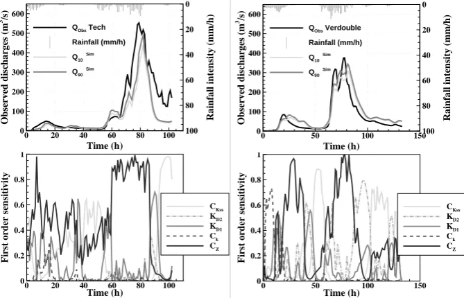
Fig. 7. (Top)Flash flood event of 15 March 2011 andQ₁₀ and Q₉₀ quintiles of simulated discharge for (left) the Tech at Pas-du-Loup (250 km2) and (right) the Verdouble at Tautavel (299 km2). (Bottom) First-order effects.

Table 4. Validation events characteristics in increasing order of specific peak flow. Mean initial soil moisture is the spatially averaged daily SIM output over a catchment.

Mean Specific Cumulated Area Validation initial soil peak flow rainfall Catchments (km2) events moisture (%) (m3s−1km−2) (mm) Beaume (Rosi`eres) 212 16 November 2006 56 1.1 111 Verdouble (Tautavel) 299 15 March 2011 52 1.2 217 Gardon (Anduze) 543 28 September 2000 56 1.4 203 Salz (Cassaignes) 144 20 December 2000 48 1.5 141 Ard`eche (Vog¨u´e) 619 3 November 2011 50 1.5 370 Ard`eche (Vog¨u´e) 619 20 October 2008 48 1.6 195 Ard`eche (Vog¨u´e) 619 31 October 2008 59 1.6 211 Tech (Pas-du-Loup) 250 15 March 2011 62 2.2 270 Gardon (Anduze) 543 18 October 2006 62 2.6 237 Gardon (Anduze) 543 8 September 2002 58 6.7 284

between soil profile storage capacity and flood event magni-tude seems nonmonotonous according to parameters sensi-tivities (Tables 4 and 7). Previous global sensitivity analysis studies already show that the model response is sensitive to CZ(Bessi`ere, 2008; Roux et al., 2011), which seems to

indi-cate that sensitivity may change little for a different optimal parameter set.

For the other parameters, relation is monotonous. The rel-ative importance of catchment infiltrability (CK) and

fric-tion in the drainage network (i.e.,KD1andKD2, channel and

overbank correction coefficients) increases with the magni-tude of the event. On the contrary, given the reduction of the proportion subsurface flow represents, the influence of sub-surface flow velocity (i.e.,CKSS)decreases with the

magni-tude of the event (Table 3).CKSSis particularly sensitive for

the Ard`eche and Salz catchments. Let us remark that the sum of first-order effectsP

i

Si is lower than one with low

stan-dard errors (Table 7) and the equality would mean that the model is additive (Saltelli et al., 2000).

5.2 Temporal evolution of first-order effects

In order to analyze the temporal dynamics of model input factors influence on the simulated discharge for the 10 flood events on six catchments, the explored variability of model response (top) and the temporally variable sensitivity indices (bottom) are represented on Figs. 5 to 8. Whatever the rain-fall patterns and volume, for some aspects of the model re-sponse, catchments behaviors characterized by the first-order

45 Time (h) F ir st o rd er s en si ti v it y

0 10 20 30 40 50 60

0 0.2 0.4 0.6 0.8 1 CKss K_D2 KD1 Ck C_Z Time (h) O b se rv ed d is ch a rg es ( m 3/s ) R a in fa ll i n te n si ty ( m m /h )

0 10 20 30 40 50 60

0 100 200 300 0 20 40 60 80 100

QObs Salz

Rainfall (mm/h) Q10 Sim Q90 Sim Time (h) F ir st o rd er s en si ti v it y

0 10 20 30 40 50 60

0 0.2 0.4 0.6 0.8 1 C_Kss KD2 KD1 Ck CZ Time (h) O b se rv ed d is ch a rg es ( m 3/s ) R a in fa ll i n te n si ty ( m m /h )

0 10 20 30 40 50 60

0 100 200 300 0 20 40 60 80 100

QObs Rosieres

Rainfall (mm/h) Q10 Sim Q90 Sim 1 2

Figure 8: (Top) Q10 and Q90 quintiles of simulated discharge on (left) 20/12/2000 for the

3

Salz at Cassaignes (144 km²), (right) 16/11/2006 for the Beaume at Rosières (212 km²). 4

(Bottom) first order effects. 5

6

Fig. 8. (Top)Q10 andQ90 quintiles of simulated discharge on (left) 20 December 2000 for the Salz at Cassaignes (144 km2), (right) 16 November 2006 for the Beaume at Rosi`eres (212 km2). (Bottom) First-order effects.

Table 5. Validation events and efficiencies in terms of1Q comparing simulated and observed peak dischargeQs_PandQo_P, and1T comparing simulated and observed peak time normalized by concentration timeT_Co, determined from Bransby formulaT_Co= 21.3L

A0.1_S0.2, whereLis channel

length (m),Ais watershed area (m2)andSis linear profile slope (m m−1).

Area Validation 1Q

= 1T=

LNP= 13(Nash+ Catchments (km2) events

Q

s p−Qop

Qo p T s p−Tpo

T_Co Nash (1−1Q)+(1−1T ))

Tech (Pas-du-Loup) 250 15 March 2011 0.15 0.32 0.70 0.73 Verdouble (Tautavel) 299 15 March 2011 0.13 0.32 0.82 0.79 Salz (Cassaignes) 144 20 December 2000 0.18 0.32 0.76 0.75

Gardon (Anduze) 543

28 September 2000 0.03 0.02 0.95 0.97 8 September 2002 0.12 0.00 0.97 0.95 18 October 2006 0.03 0.15 0.60 0.80

Beaume (Rosi`eres) 212 16 November 2006 0.32 0.10 0.64 0.75

Ard`eche (Vog¨u´e) 619

20 October 2008 0.02 0.02 0.93 0.96 31 October 2008 0.13 0.04 0.87 0.89 3 November 2011 0.23 0.40 0.85 0.73

Average 0.13 0.17 0.81 0.83

sensitivity indices are similar. First, before rainfall starts,CZ,

CKSSandKD1– i.e., soil depths, lateral subsurface flow and

main channel roughness – explain most of the variability be-cause the initial soil water content (above 48 %, Table 4) ac-tivates subsurface flow and exfiltration in the drainage net-work. Only the main channel represented by KD1 is

con-cerned by these small amounts of water at the outlet (a few m3s−1).

Then we can distinguish the 16 November 2006 event at Rosi`eres (Fig. 8, right), the smallest one in terms of

spe-cific discharge, from the nine others obviously activating all model flow components. This event is underestimated by MARINE and is characterized by an important sensitivity to CZ, especially at peak time and early recession (11 to 22 h)

of the hydrograph.CKandKD1play a small role during the

rising limb. Moreover, while the influence of the parameter driving infiltrability (i.e.,CK)is low, subsurface flow

repre-sented by parameterCKSSplays an important role (10 % of

total variance). Only “minor flow components” are activated

Table 6. Gardon d’Anduze: 8 September 2002 flash flood event, first-order effects and standard error averaged in time, and first-order metamodelR2for different sampling ranges around nominal parameter values.

α Si1 CZ Si1 CK Si1CKSS Si1KD1 Si1KD2 Sum (Si1) Sum (Si1 std err) R2Sum (Si1) ±5 % 0.392 0.183 0.119 0.198 0.091 0.983 0.020 0.972 ±10 % 0.413 0.170 0.109 0.195 0.079 0.967 0.028 0.975 ±15 % 0.376 0.169 0.117 0.196 0.081 0.940 0.030 0.971

Table 7. First-order effects (–), standard error and first-order metamodelR2averaged in time for each event of the validation set sorted in ascending order of specific peak flow. For each event 1024 events are analyzed.

Area Sum Sum

Catchments (km2) Validation events Si1CZ Si1 CK Si1CKSS Si1KD1 Si1KD2 (Si1) (Si1stdev) R2

Beaume (Rosi`eres) 212 16 November 2006 0.73 0.00 0.23 0.00 0.00 0.979 0.038 0.99

Verdouble (Tautavel) 299 15 March 2011 0.36 0.06 0.22 0.13 0.22 0.992 0.021 0.97

Gardon (Anduze) 543 28 September 2000 0.49 0.01 0.17 0.20 0.07 0.943 0.056 0.94

Salz (Cassaignes) 144 20 December 2000 0.29 0.03 0.42 0.11 0.09 0.941 0.038 0.99

Ard`eche (Vog¨u´e) 619 3 November 2011 0.51 0.04 0.27 0.05 0.13 0.997 0.019 0.98

Ard`eche (Vog¨u´e) 619 20 October 2008 0.47 0.15 0.23 0.07 0.07 0.993 0.016 0.99

Ard`eche (Vog¨u´e) 619 31 October 2008 0.33 0.04 0.49 0.04 0.07 0.967 0.011 0.99

Tech (Pas du Loup) 250 15 March 2011 0.49 0.02 0.26 0.16 0.02 0.948 0.046 0.94

Gardon (Anduze) 543 18 October 2006 0.57 0.00 0.15 0.14 0.08 0.947 0.035 0.93

Gardon (Anduze) 543 8 September 2002 0.41 0.17 0.11 0.20 0.08 0.966 0.028 0.98

Average 0.43 0.05 0.24 0.11 0.08 0.92 0.034 0.92

for that catchment and event – i.e., moderate solicitation of flow components without floodplain invasion.

At the beginning of rainfalls, and during heavy rainfalls, a similar general sensitivity pattern can be found for the nine other events (Figs. 5 to 8); most flow components are ac-tivated: infiltration, lateral subsurface flow, hillslope runoff, main channel and floodplain flow. The temporal evolution of parameter’s influence involves in the following order the different processes: infiltrability, transfer and limitation by maximum soil storage capacity. In fact,CK determining

in-filtration capacity is sensitive for significant rainfall intensity variations (Fig. 5 at 15 h, Fig. 6 at 47 and 57 h, Fig. 7 (right) at 8 h, Fig. 8 (left) at 25 h). Before the hydrograph’s rising limb, KD1, the main channel friction coefficient, drives the

uncer-tainty, and then soil depth coefficientCZ is sensitive, which

defines cells total storage capacity. This highlights sensitivity to the soil volume, which influences saturation dynamics and so on to water volumes partitioning among the catchment. Let us remark that CZ explains more than 80 % of model

output variance when most hydrographs are peaking. However, the presence of some peaks ofCKSSinfluence

during simulations (Fig. 5 around 10, 60 and 160, 210 and 240 h; Fig. 6 around 15, 55 and 87 h; Fig. 7 (left) around 50 h, (right) around 52 h; Fig. 8 (left) around 15 h) can be explained by a significant contribution of subsurface flow. Indeed,CKSSis the adjustment parameter of soil lateral

con-ductivity for subsurface flow. It can have an impact on sim-ulated discharge by modifying the distribution of soil

wa-ter content and thus infiltration dynamics. During recession, CKSSsensitivity generally increases, which can show the role

of subsurface in recession dynamics according to the model. Let us consider the high CKSS sensitivities explaining

more than 80 % of model output variance for slow recessions in the case of 31 October 2008 and 3 November 2011 floods on the Ard`eche at Vog¨u´e for instance (Fig. 5), as for slow hy-drograph rising limb in the case of the 15 March 2011 flood of the Verdouble at Tautavel (Fig. 7, right, at 51 h) or the 20 December 2000 flood of the Salz at Cassaignes (Fig. 8, left, between 10 and 20 h)

KD2the overbank roughness coefficient is sensitive during

late rising and early falling limbs, when saturation is high and a huge amount of water is transferred to the outlet by overbank flow (Fig. 5 around 20, 90 h and between 170 and 225 h; Fig. 6 around 35, 67 and 115 h; Fig. 7 (left) around 90 h, (right) around 40, 65 and 100 h; Fig. 8 (left) around 45 h).

Finally, it can be remarked that in the case of the 8 Septem-ber 2002 extreme event at Anduze, a complex catchment be-havior reflected by quickly variable and marked sensitivities is caused by an extreme storm in the very lower part of the catchment causing short response delays (more than 400 mm cumulated rainfall on half of the catchment with maxima greater than 700 mm located close to the outlet). On the con-trary, the 18 October 2006 and 28 September 2000 gener-ating storms hit the medium or upper part of the Gardon d’Anduze catchment with less violence. For these longer rain

46 Time (h)

1

S

u

m

(

Si

)

0 50 100 150 200 250

0 0.2 0.4 0.6 0.8 1

1-Sum(Si)

Time (h)

O

b

se

rv

ed

d

is

ch

a

rg

es

(

m

3/s

)

R

a

in

fa

ll

i

n

te

n

si

ty

(

m

m

/h

)

0 50 100 150 200 250

0 500 1000

1500 0

20 40

60

80 100

QObs 3evs Vogüé

Rainfall (mm/h)

Q10 Sim

Q90 Sim

1 2

Figure 9: (Top) Ardèche at Vogüé, 20/10/2008, 31/10/2008 and 03/11/2011 flash flood 3

events and quintiles Q10 and Q90 of simulated discharge. (Bottom) −

∑

i i S

1 . 4

Fig. 9. (Top) Ard`eche at Vog¨u´e: 20 October 2008, 31 October 2008 and 3 November 2011 flash flood events and quintilesQ10andQ90of simulated discharge. (Bottom) 1−P

i

S_i.

47 Time (h)

1

S

u

m

(

Si

)

0 20 40 60 80 100 120

0 0.2 0.4 0.6 0.8 1

1-Sum(Si)

Time (h)

O

b

se

rv

ed

d

is

ch

a

rg

es

(

m

3/s

)

R

a

in

fa

ll

i

n

te

n

si

ty

(

m

m

/h

)

0 50 100

0 1000 2000 3000 4000

5000 0

20

40 60

80 100

QObs 3evs Gardon

Rainfall (mm)

Q10 Sim

Q90 Sim

1

2

Figure 10: (Top) Gardon at Anduze, 28/09/2000, 08/09/2002 and 18/10/2006 flash flood 3

events and quintiles Q10 and Q90 of simulated discharge. (Bottom) −

∑

i i S

1 . 4

Fig. 10. (Top) Gardon at Anduze: 28 September 2000, 8 September 2002 and 18 October 2006 flash flood events and quintilesQ10andQ90 of simulated discharge. (Bottom) 1−P

i

Si.

events the temporal sensitivities vary more slowly. Moreover, for sensitivity peaks ofCZ and thenKD1,KD2, (Fig. 6

be-tween 20 and 30 h, and bebe-tween 95 and 122 h) corresponding to rainfall peaks responses, CZ sensitivity stays above the

other during the flood. This can be attributed to a catchment spatio-temporal dampening effect: when a storm hits catch-ment headwaters, a larger soil storage volume is involved in flood generation.

5.3 Analysis of temporal interaction effects

Using variance-based sensitivity analysis methods, an essen-tial aspect is that the estimatedS_i0shave interesting normal-ization properties. Indeed, from Eq. (5) normalized byV (Y ) and with Eq. (6), the sum of nicely scaled sensitivity mea-sures between 0 and 1 can be written as

1=X

i

Si+

X

i

X

j

Sij+. . .+S1,2,...,k. (7)

48

0 20 40 60 80 100

0 0.2 0.4 0.6 0.8 1

1-Sum(Si)

Time (h) O b se rv ed d is ch a rg es ( m 3 /s ) R a in fa ll i n te n si ty ( m m /h )

0 20 40 60 80 100

0 200 400 600 0 20 40 60 80 100

QObs Tech

Rainfall (mm/h) Q10 Sim Q90 Sim Time (h) 1 S u m ( Si )

0 50 100 150

0 0.2 0.4 0.6 0.8 1

1-Sum(Si)

Time (h) O b se rv ed d is ch a rg es ( m 3 /s ) R a in fa ll i n te n si ty ( m m /h )

0 50 100 150

0 100 200 300 400 500 600 700 0 20 40 60 80 100

QObs Verdouble

Rainfall (mm/h) Q10 Sim Q90 Sim

1

2

Figure 11: (Top) 15/03/2011 flash flood event and Q

and Q

quintiles of simulated

3

discharge on (left) the Tech at Pas-du-Loup and (right) the Verdouble at Tautavel.

4

(Bottom)

−

∑

i i

S

1

.

5

Fig. 11. (Top) Flash flood event of 15 March 2011 andQ10andQ90quintiles of simulated discharge for (left) the Tech at Pas-du-Loup and (right) the Verdouble at Tautavel. (Bottom) 1−P

i

Si.

49

0 20 40 60 80 100 120

0 0.2 0.4 0.6 0.8 1

1 - Sum(Si)

Time (h) O b se rv ed d is ch a rg es ( m 3 /s ) R a in fa ll i n te n si ty ( m m /h )

0 20 40 60 80 100 120

0 50 100 150 200 250 300 0 20 40 60 80 100

Q_Obs Salz

Rainfall (mm/h) Q10 Sim Q90 Sim Time (h) F ir st or d er s en si ti vi ty

0 20 40 60

0 0.2 0.4 0.6 0.8 1

1 - Sum(Si)

Time (h) O b se rv ed d is ch a rg es ( m 3 /s ) R a in fa ll i n te n si ty ( m m /h )

0 20 40 60

0 100 200 300 0 20 40 60 80 100

QObs Rosières

Rainfall (mm/h) Q10 Sim Q90 Sim

1

2

Figure 12: (Top) Q

and Q

quintiles of simulated discharge on (left) 20/12/2000 for the

3

Salz at Cassaignes, (right) 16/11/2006 for the Beaume at Rosières. (Bottom)

−

∑

i i

S

1

.

4

Fig. 12. (Top)Q10andQ90quintiles of simulated discharge on (left) 20 December 2000 for the Salz at Cassaignes and (right) 16 Novem-ber 2006 for the Beaume at Rosi`eres. (Bottom) 1−P

i

Si.