Improving streamflow predictions at ungauged locations with real time updating: application of an EnKF based state parameter estimation strategy

www.hydrol-earth-syst-sci.net/18/3923/2014/ doi:10.5194/hess-18-3923-2014

© Author(s) 2014. CC Attribution 3.0 License.

Improving streamflow predictions at ungauged locations with

real-time updating: application of an EnKF-based state-parameter

estimation strategy

X. Xie1, S. Meng1, S. Liang1,2, and Y. Yao1

1_{State Key Laboratory of Remote Sensing Science, College of Global Change and Earth System Science,} Beijing Normal University, Beijing, China

2_{Department of Geographical Sciences, University of Maryland, College Park, Maryland, USA}

Correspondence to: X. Xie ([email protected])

Received: 13 October 2013 – Published in Hydrol. Earth Syst. Sci. Discuss.: 8 November 2013 Revised: 27 August 2014 – Accepted: 9 September 2014 – Published: 7 October 2014

Abstract. The challenge of streamflow predictions at un-gauged locations is primarily attributed to various uncer-tainties in hydrological modelling. Many studies have been devoted to addressing this issue. The similarity regionaliza-tion approach, a commonly used strategy, is usually limited by subjective selection of similarity measures. This paper presents an application of a partitioned update scheme based on the ensemble Kalman filter (EnKF) to reduce the predic-tion uncertainties. This scheme performs real-time updating for states and parameters of a distributed hydrological model by assimilating gauged streamflow. The streamflow predic-tions are constrained by the physical rainfall-runoff processes defined in the distributed hydrological model and by the cor-relation information transferred from gauged to ungauged basins. This scheme is successfully demonstrated in a nested basin with real-world hydrological data where the subbasins have immediate upstream and downstream neighbours. The results suggest that the assimilated observed data from down-stream neighbours have more important roles in reducing the streamflow prediction errors at ungauged locations. The real-time updated model parameters remain stable with reason-able spreads after short-period assimilation, while their es-timation trajectories have slow variations, which may be at-tributable to climate and land surface changes. Although this real-time updating scheme is intended for streamflow predic-tions in nested basins, it can be a valuable tool in separate basins to improve hydrological predictions by assimilating multi-source data sets, including ground-based and remote-sensing observations.

1 Introduction

The streamflow prediction plays a central role in hydrology because it is an important element for water resources man-agement, the design of hydraulic infrastructures and flood risk mapping (Srinivasan et al., 2010). Because it is an impor-tant component in the terrestrial water budget, streamflow is also a direct diagnostic variable measuring the impact of cli-mate changes and human activities that act on a given water-shed. Streamflow prediction depends highly on reliable hy-drological data and sophisticated hyhy-drological models. How-ever, hydrological data are often insufficient due to ungauged or poorly gauged basins in many parts of the world (Siva-palan, 2003). Because of the scarcity of data, hydrological modelling is also plagued by various sources of uncertain-ties. To reduce uncertainties from those hydrological data and hydrological modelling, the International Association of Hy-drological Sciences (IAHS) launched an initiative on Predic-tions in Ungauged Basins (PUB) (Sivapalan, 2003; Sivapalan et al., 2003).

snowmelt-runoff responses. This progress has fostered spe-cific problem areas in the field: uncertainty quantification with respect to model input forcing, model structures and pa-rameters (Ajami et al., 2007; Vrugt et al., 2008; Gupta et al., 2012). To reduce the uncertainty from model parameters, one common practice is the parameter calibration by adjust-ing model parameters to make the simulated water discharges correspond to the observations (typically the data from the outlet of a watershed) (Duan et al., 1992, 1994). However, a calibrated parameter set with acceptable streamflow simula-tion performance at the watershed outlet does not guarantee the performance at interior locations (Zhang et al., 2008).

The essence of PUB is to transfer information from neigh-bouring basins to the basins of interest (Sivapalan et al., 2003). Such process is generally referred to as hydrologi-cal regionalization, based on either regression methods or measurable distances (with respect to physical similarity or spatial proximity) between gauged and ungauged locations (Hrachowitz et al., 2013). Regionalization techniques regard-ing model parameters are popular for discharge prediction in ungauged basins. Merz and Blöschl (2004) evaluated the performance of various regionalization methods for parame-ters of a conceptual catchment model, determining that spa-tial proximity is able to represent the unknown controls on the runoff regime and the relationships of model parameters within neighbouring basins. Sellami et al. (2014) presented a model parameter regionalization approach based on physical similarity between gauged and ungauged catchments, indi-cating that similar hydrological behaviour may appear due to physically similar catchments in the same geographic and climatic region. Parajka et al. (2013) reported that the spa-tial proximity and geostatistics probably perform better than the regression or regionalization with a simple averaging of model parameters from gauged catchments. One drawback of the regionalization of model parameters is that it often con-fronts an arbitrary criterion for selecting the “behavioural” model parameter sets from the gauged catchment (Sellami et al., 2014). Hrachowitz et al. (2013) provides a comprehen-sive review of the parameter regionalization and catchment similarity.

In addition to those parameter regionalization approaches, newly developed data assimilation methods are also encour-aging and are capable to address some issues associated with PUB. They are generally based on physical correlations be-tween the neighbouring basins, and they can combine multi-source observations to transfer information from gauged to ungauged basins (Sivapalan et al., 2003; Troch et al., 2003; Chen et al., 2011). As a typical sequential data assimila-tion approach, the ensemble Kalman filter (EnKF) is popu-lar in hydrology (Reichle et al., 2002; Evensen, 2003, 2009). The EnKF is attractive in hydrology primarily because it can perform real-time updating with simple implementation and it considers various uncertainties in modelling and observa-tions (Blöschl et al., 2008). The feature of real-time updating is very important for flood forecasting (Norbiato et al., 2008).

In some current applications, EnKF is mainly dedicated to dynamic state estimations in which the model parameters are defined with prior values or calibrated in advance (Vrugt et al., 2005; Clark et al., 2008).

The EnKF method also provides a general framework to perform state-parameter estimation which is the core of PUB issues. It is has been successfully used for parameter esti-mation of hydrological models. Moradkhani et al. (2005b) proposed a dual state-parameter estimation of hydrological models and made an acceptable application of this method for a lumped hydrological model. Wang et al. (2009) pre-sented three constrained schemes with EnKF to prevent the violation of parameter physical constraints. Most of these studies performed parameter estimations for lumped hydro-logical models with a small number of parameters to be es-timated. Xie and Zhang (2010) successfully demonstrated a joint state-parameter estimation based on the EnKF for a distributed hydrological model, i.e. Soil and Water Assess-ment Tool (SWAT), focusing on one dominant parameter in SWAT. For multiple types of parameter estimation, Xie and Zhang (2013) developed a partitioned update scheme and in-dicated the potential of this scheme for streamflow predic-tions in ungauged basins based on distributed hydrological models.

In this study, we present the application of the partitioned update scheme to improve streamflow predictions in un-gauged locations by assimilating un-gauged streamflow. This data assimilation algorithm is fully coupled with the dis-tributed hydrological model, i.e. SWAT. The state vector and parameters in ungauged subbasins are estimated when information is transferred from gauged subbasins. To our knowledge, this study is the first one which explicitly em-ploys a data assimilation method with state-parameter esti-mation to improve streamflow predictions in ungauged loca-tions. Although a few applications of data assimilation meth-ods are dedicated to streamflow predictions based on dis-tributed models (Clark et al., 2008; Chen et al., 2011; Lee et al., 2012; Rakovec et al., 2012; McMillan et al., 2013), the model parameter estimation, which is important for PUB, is not systematically considered. In addition to the EnKF-based scheme, note that the other data assimilation methods, e.g. the particle filter (Moradkhani et al., 2005a; DeChant and Moradkhani, 2012), the Particle-DREAM (Vrugt et al., 2013) and the Maximum Likelihood Ensemble Filter (Tran et al., 2014), may also be optional for state-parameter esti-mation.

gauged locations on streamflow predictions. Finally, conclu-sions are given in the last section.

2 Methodology

2.1 EnKF-based state and parameter estimation scheme

To describe the information transfer process from gauged to ungauged locations, we define a joint state vectorXthat contains gauged (xg) and ungauged (xu) states:X= [xg, xu]. Moreover, we consider the diagnostic variables, i.e. the wa-ter discharge and the evapotranspiration, as model states and include them in the vectorXto perform streamflow updating in the data assimilation. The joint state vectorXand the pa-rameter vectorθestimation at timetare conditioned on mea-surements (yt) from gauged basins. The information transfer

process, i.e. the posterior probability density function (pdf)

p(Xt,θt|yt), can be expressed within Bayes’ framework,

p(Xt,θt|yt)∝p( yt|Xt,θt)·p(Xt,θt|Xt−1,θt−1), (1) where p( yt|Xt,θt) is the likelihood function of

mea-surements given model estimations at time t. Moreover,

p(Xt,θt|Xt−1,θt−1) is the prior pdf of Xandθ at timet that represents model forecasting and parameter evolutions.

The updating framework defined in Eq. (1) is well in-cluded in and effectively solved by sequential data assim-ilation strategies – typically, the EnKF strategy (Evensen, 1994). The EnKF strategy operates sequentially with a fore-cast step and a filter update step. In the forefore-casting process, uncertainty propagation is characterized by an ensemble of model realizations:

X_ti−=M(X_ti+₋₁,θi_t−, ui_t)+ωi_t,ωi_t∼N (0, Wt), (2)

i=1,2, . . . N,

where “−” and “+” denote the forecast and analysis for the state vectorsXand the parameter vectorθ,tis the time step,

uis the input forcing vector, andNis the ensemble size. The model error vector ωis assumed to follow a Gaussian dis-tribution with zero mean and covarianceWt. Equation (2) is

a general expression with representative errors for all state variables. In implementation, one may define errors for only a few of the state variables (e.g. soil moisture) to reflect real-istic modeling uncertainties. Detailed prescription of the er-rors will be given in Sect. 3.2.

Prior to model forecasting using Eq. (2), the model pa-rameters can be perturbed, similar to the forecast of the state vector, to avoid the shrinkage of the parameter ensemble dur-ing the updatdur-ing (Wang et al., 2009). However, the parame-ter perturbation is susceptible to over-dispersion in sampling (Moradkhani et al., 2005b). A kernel smoothing technique is effective to address the over-dispersion while maintaining a reasonable ensemble spread for the parameters (Liu, 2000;

Moradkhani et al., 2005b; Xie and Zhang, 2013). This tech-nique is briefly expressed as

θi_t−=αθ_ti+₋₁+(1−α)θ¯+_t−1+τi_t,τi_t∼N (0, Tt), (3)

¯

θ+_t−1= 1

N

N

X

i=1

θi_t+₋₁, (4)

Tt=h2var θ+_t−1, (5)

whereαis the shrinkage factor typically within [0.95, 0.99],

h is the smoothing factor, and Tt is the covariance

con-strained by the ensemble variance var θ+_t . The smoothing factorhis defined as

√

1−α2 _{to maintain equal variances} of the parameter before and after the perturbation. This ker-nel smoothing technique has been discussed based on syn-thetic cases (Liu, 2000; Moradkhani et al., 2005b; Xie and Zhang, 2013), so we do not provide any more experiments to demonstrate the properties of the kernel smoothing. The pre-scription of the shrinkage factorαis subject to trial and error experimentation, but it has limited impact on the parameter estimation (An illustrative case was shown in the response to the reviewers’ comments at version 4 of this paper). In this study, it is specified with 0.98 according to the suggestions by Moradkhani et al. (2005b) and Xie and Zhang (2013).

With the forecast of the states and parameters, the filter up-date step is performed when observations are available. This updating is actually the solving process for Eq. (1). Here we intentionally create an explicit expression of the updating for gauged and ungauged states and parameters:





xi_g+_,t xi_u+_,t

θi_t+ 

= 



x_gi−_,t x_ui−_,t

θi_t− 

+Kt·

y_ti−H x_gi+_,t, (6)

whereyi_t is the observation vector, which is appropriately perturbed using covariance ofRto account for uncertainties in observations, andH is the observation operator and it is linear in this study. The Kalman gain matrix Kt is expressed

as

Kt =





cov(xg,t, xg,t) cov(xg,t, xu,t) cov(xg,t,θt)



· cov(xg,t, xg,t)+R −1

, (7)

where cov(·) is the covariance operator that is computed from the ensembles of states and parameters. Note that the size of the matrix Kt isn×m, wherenis the total number of state

variables and parameters andmis the number of observa-tions.

because it allows for parameter dynamics and performs the parameter evolution. Specifically, model parameters are as-sumed as an extension of state variables and they can travel slowly with time, in response to changes in environmental forcing inputs (Liu and Gupta, 2007). Like the model state forecasting, the parameters are perturbed/evolved using the kernel smoothing technique. In this way, the evolution of model parameters is consistent with the forecasting of model state variables. Thus the model parameters can be appended to the state vector (Moradkhani et al., 2005b; Xie and Zhang, 2010, 2013). When observations are available, the parame-ters are updated along with state variables by assimilating these observations. Therefore, their estimates are expected to converge to the “correct” posterior target distribution (Xie and Zhang, 2013). This technique has been successfully used in many cases for real-time state and parameter estimation (Moradkhani et al., 2005b; Wang et al., 2009; Xie and Zhang, 2010, 2013).

We can see that EnKF provides a general framework to transfer information from gauged to ungauged basins. How-ever, when used for parameter estimations in distributed hy-drological models, it is vulnerable to corruption due to spu-rious covariance computation in Eq. (7), primarily resulting from a large degree of freedom for high-dimensional vec-tors of the augmented state. To relieve this problem, Xie and Zhang (2013) proposed a partitioned forecast-update scheme (PU_EnKF) that is inspired by the dual state-parameter es-timation algorithm (Moradkhani et al., 2005b). In the par-titioned forecast-update scheme, the parameter set of a hy-drological model is partitioned into different types (Nptypes in total) based on their sensitivities. Each type is estimated in an individual loop by repeated forecasting and updating. Here, the parameter type maintains an aggregation conno-tation. A parameter type can contain only one parameter (e.g. for lumped hydrological models) or many parameters associated with the same number of computational units in distributed hydrological models. For example, the parameter CN2in SWAT (will be introduced in Sect. 2.2) is considered as a parameter type.

At time t, the PU_EnKF is iteratively applied as follows forNploops:

I. Perform parameter evolution using Eq. (3) for thejth parameter type, producing a new ensemble of parame-ters.

II. Run the modelN times following Eq. (2) to obtain en-semble predictions for gauged and ungauged state vari-ables. In the prediction, thejth parameter type is pre-scribed with a member of the ensemble produced in step I, while the others are set with the ensemble means that are estimated from previous loops at this time step and from the previous time step.

III. Compute the Kalman gain matrix using Eq. (7) based on the ensembles of states and parameters when obser-vations become available at timet.

IV. Update the state vector and thejth parameter type using Eq. (6).

V. Compute the ensemble means of thejth parameter type. The means are the estimates of the parameters and will be used in step II in the subsequent loops to estimate the other parameter types.

VI. Return to step I ifj <Np. Otherwise, go to the next time stept+1. The updated state vector from the loopj=

Npis considered as estimates of gauged and ungauged state variables; and all estimates of parameters are also obtained.

We can see that the partitioned update scheme employs an iterative algorithm to update each parameter type at each time step – not only is one parameter considered at a time. At timet, the new estimated parameter values from previ-ous loops are used for the model forecasting (Eq. 2) in the current loop in which a target parameter type (thejth param-eter type) is estimated. This iterative update is expected to push the estimates towards their optimal values. Therefore, this scheme is suitable for distributed hydrological models to estimate high-dimensional parameters. Its capability has been demonstrated using synthetic cases and it has been suc-cessfully used in a real watershed for state and parameter es-timation (Xie and Zhang, 2013). In this study, we apply this scheme to improve the streamflow prediction in ungauged sites and to estimate model parameters.

2.2 Model description

The distributed hydrologic model, SWAT, is a basin-scale hydrological model developed by the USDA Agricultural Research Service (Arnold et al., 1998; Arnold and Fohrer, 2005). In implementation of SWAT, a basin is partitioned into multiple subbasins that are then divided into hydrologic response units (HRUs), which consist of unique land cover, management, and soil characteristics (Neitsch et al., 2001; Gassman et al., 2007). The HRUs are the basic computational units in which the overall hydrologic balance is simulated, in-cluding precipitation partitioning, surface runoff generation, evapotranspiration (ET), soil water and groundwater move-ment.

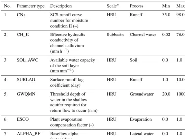
Table 1. Model parameters to be estimated in data assimilation.

No. Parameter type Description Scale∗ Process Min Max

1 CN2 SCS runoff curve number for moisture condition II (–)

HRU Runoff 35.0 98.0

2 CH_K Effective hydraulic conductivity of channels alluvium (mm h−1)

Subbasin Channel water 0.02 76.0

3 SOL_AWC Available water capacity of the soil layer (mm mm−1)

HRU Soil 0.0 1.0

4 SURLAG Surface runoff lag coefficient (day)

HRU Runoff 1.0 10.0

5 GWQMN Threshold depth of water in the shallow aquifer required for return flow to occur (mm)

HRU Groundwater 20.0 1000.0

6 ESCO Plant evaporation compensation factor (–)

HRU Evaporation 0.0 1.0

7 ALPHA_BF Baseflow alpha factor (day)

HRU Lateral water 0.0 1.0

∗_{The hydrologic variables are with respect to the scales to reflect the related hydrologic processes.}

capacity to dominate redistribution of water between layers. By infiltration or percolation, a fraction of water below the soil profile enters groundwater storage as recharge and is par-titioned between shallow and deep aquifers. Base flow from the shallow aquifer is also routed to river channels. Details regarding these processes can be found in the SWAT user’s manual (Neitsch et al., 2001).

SWAT contains a large number of spatially varying pa-rameter types to be prescribed before hydrologic simula-tion and predicsimula-tion. These parameters consist of the surface roughness, soil properties, land-cover pattern and hydraulic conditions of the river channel. Although their default val-ues can be prescribed according to lookup tables, the op-timal values must be calibrated on the basis of modelling behaviour and observations. To reduce the number of cali-brating parameters, a sensitivity analysis is usually required (van Griensven et al., 2006). Considerable effort has been devoted to sensitivity analysis for SWAT; several parameters are recognized as the most influential ones that dominate the model behaviour (Holvoet et al., 2005; Muleta and Nicklow, 2005; van Griensven et al., 2006). Based on these studies, seven parameters (also called parameter types) are selected and shown in Table 1. They underpin different hydrologic processes in a basin involving the surface runoff, soil water, baseflow, groundwater, evapotranspiration and channel water processes. Their ranges are determined in terms of the lookup

tables (Neitsch et al., 2001) and the specific soil and land use properties of the Zhanghe River basin (Post and Jakeman, 1999).

In addition to these sensitive parameter types, ten hydro-logic variables are selected to be updated in data assimilation (Table 2). They can be divided into three groups: (1) quick water storage (marked with QW in Table 2) regarding sur-face runoff, (2) slow water storage (marked with SW) associ-ated with baseflow and groundwater flow and soil moisture, and (3) river channel storage (marked with CW) and flow. The first nine variables are the dynamic states that character-ize water storage status in HRUs or subbasins and partially influence the diagnostic variables, i.e. ET and the water dis-charge (Qr). Therefore, along with both outputs, these states should be updated to guarantee consistent model behaviour. In this study, ET is excluded from the state vector because there are no ET observations and its passive update in data assimilation does not impact other state estimations.

Table 2. Dynamic hydrologic states and outputs to be updated in data assimilation.

Variable Description Scale1 Storage2

Qsurfstor Amount of surface runoff stored or lagged (mm) HRU QW

Qlatstor Amount of lateral flow stored or lagged (mm) HRU QW

Qpregw Amount of groundwater flow into the main channel (mm) HRU QW

Wsol Amount of water stored in the soil layer for each HRU (mm) HRU×Nlay SW

SM Amount of water stored in soil profile (mm) Subbasin SW

Qshall Amount of shallow water stored or lagged (mm) HRU SW

Qrchrg Amount of recharge entering the aquifer (mm) HRU SW

Wr Amount of water stored in the reach (m3) Subbasin CW

Wb Amount of water stored in the bank (m3) Subbasin CW

Qr Amount of water flow out of reach (Streamflow, m3s−1) Subbasin CW

1_{This column indicates the scale at which each variable is simulated.N}

layis the number of soil layers (Nlay=4for this study), and

HRU×Nlaymeans the soil profile of each HRU is partitioned intoNlaylayers.2This column denotes water storage condition for

each variable: QW, quick water storage; SW, slow water storage; and CW, river channel storage.

few successful applications (Xie, 2013; Xie and Zhang, 2010, 2013). Therefore, such a coupled SWAT-EnKF data assimi-lation platform is expected to be more powerful and widely used for real-time hydrological predictions. SWAT requires a significant amount of data including model input and system response data (e.g. streamflow, evapotranspiration), which seems not consistent with effort of predictions in ungauged basins. But this issue can be eased to some degree because streamflow data from just a few locations downstream (e.g. the outlet) can favour estimation for the entire basin by the data assimilation scheme used in this study.

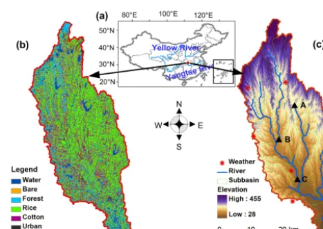
3 Application to a real case 3.1 Study area and database

The data assimilation scheme is applied in the Zhanghe River basin in Hubei Province, China (Fig. 1). The Zhanghe drains an area of 1129 km2, and the elevation difference between the north and the south is more than 400 m. It has a typi-cal subtropitypi-cal climate with an annual mean temperature of 17◦C. The annual rainfall in the catchment is approximately 970 mm per year, although rainfall varies substantially from year to year depending upon the monsoon strength. This basin is actually an agricultural irrigation area and its tivated area accounts for 59 %. Paddy rice is the primary cul-tivated plant, which, from May to August, requires irriga-tion water from the Zhanghe reservoir and thousands of local ponds. Owing to intense human activities, including culti-vation, irrigation and drainage, streamflow prediction in this basin is a challenge with large uncertainties (Cai, 2007; Xie and Cui, 2011).

We chose the Zhanghe River basin as a study area because there are sufficient data sets associated with weather condi-tions, land use and soil properties, and hydrological informa-tion. This area has been chosen for a few modelling studies

Figure 1. Zhanghe River basin in China (a), the land use (b) and subbasin distribution with DEM (c).

according to calibrated rating curves, daily streamflow data for the period 2003–2006 are available.

The Zhanghe River basin is divided into 20 subbasins based on a digital elevation model (DEM) with a resolu-tion of 90 m (Fig. 1c). Thereafter, 98 HRUs are obtained ac-cording to land use and the soil map. With this delineation, Gauge A drains runoff from a source subbasin, Gauge B drains four, Gauge C drains ten, and Gauge D drains all the basins.

3.2 Error quantification

The success of ensemble-based data assimilation methods depends partly on ensemble generations to quantify errors from model input forcing, parameters and model structures. Moreover, quantifying observation errors is also critical to account for uncertainties from measurements and deriva-tions. Due to the dynamics of the SWAT model, the er-rors/uncertainties from the input forcing, parameters and the model structure are transferred to the water storages (e.g. soil moisture and channel storages) and diagnostic variables (e.g. streamflow). Although 10 selected variables require updating in SWAT, two of them (i.e. soil moisture and streamflow) are perturbed in this study to represent the modelling uncertain-ties, because the other variables are internal and their uncer-tainties are transferred to the soil moisture and the simulated streamflow (Xie and Zhang, 2013). Precipitation as a major forcing input is also perturbed to represent the uncertainty probably derived from weather forecasting and other sources. Perturbations to the above three variables are conducted based on zero-mean Gaussian distributions. The standard de-viation (σ) for SWAT-simulated soil moisture is set as 0.03 m3m−3as suggested by Chen et al. (2011). The standard de-viations for streamflow and precipitation are assumed to be proportional to their values (Clark et al., 2008),

σx=ηx·x, (8)

where η is the fractional factor of the standard devia-tion to the variable x. Thus, there are three fractional fac-tors corresponding to the simulated streamflow (ηQm), ob-served streamflow (ηQo) and precipitation (ηp). Therefore the PU_EnKF scheme used in this study is also applicable to hydrological prediction when measured rainfall data are unavailable but could be derived from various sources (e.g. weather forecasting). With this error quantification, the three standard deviations vary with time, depending on the magni-tudes of the four variables.

These fractional factors should not only represent the re-lated uncertainties in modelling and the observations but also produce ensemble streamflow predictions with reasonable ensemble spread (Clark et al., 2008). Based on the uncer-tainty analysis by Xie and Cui (2011), the prediction errors with the SWAT model are more than 10 % of the variables due to the irrigation and drainage practices in the Zhanghe River basin; the measurement of precipitation also has the

Table 3. Fractional factors used to perturb the precipitation (ηp), simulated streamflow (ηQm) and the observed streamflow (ηQo).

Distribution parameter ηp ηQm ηQo

Values of fractional factor 0.10 0.15 0.10

same level of uncertainty. Therefore, various combinations of factor values are evaluated by running the data assimila-tion procedure. Table 3 presents the final choice of the three fractional factors.

Note that the error quantification remains challenging for land surface data assimilation. A few newly developed ap-proaches may be a good attempt, e.g. adaptive filtering (Crow and Reichle, 2008; Reichle et al., 2008). However, we quan-tify the model and observation uncertainties in terms of an experiential and practical perspective in which large storm events normally induce larger uncertainties in modelling and observations. Moreover, an overestimation of uncertainties is a better practice than underestimation to avoid the ensemble shrinkage (Crow and Van Loon, 2006; Clark et al., 2008).

3.3 Assimilation set-up and scenario design

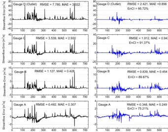
Figure 2. Streamflow prediction errors from the control-run simulation (left column) and the data assimilation of scenario ASS_D (right column), i.e. only the observed streamflow from Gauge D (outlet) is assimilated to update model states and parameters.

precipitation), and variables of channel water storage (CW) are updated at every time step.

To demonstrate the improvement of streamflow prediction in ungauged locations, we only assimilate streamflow from one or two of the four gauges, and the remaining gauges, regarded as pseudo-ungauged locations, are used to validate the performance of data assimilation. Three scenarios with different combinations of data from the four gauges are de-signed:

I. ASS_D: the observed data of streamflow from Gauge D are assimilated; Gauges A, B and C are assumed as pseudo-ungauged. This scenario is similar to a common calibration practice for which only the outlet (Gauge D) discharge data are employed to calibrate the parameters and to extrapolate streamflow of ungauged subbasins. II. ASS_BD: the observed data of streamflow from Gauge

B and D are assimilated; the other two are regarded as pseudo-ungauged subbasins. This scenario adds the data from Gauge B at the upstream in this basin based on scenario ASS_D.

III. ASS_AB: the observed data of streamflow only from Gauge A and B are assimilated. This scenario only uses the streamflow from the two gauges in the upstream sub-basins.

3.4 Prediction in ungauged locations

Ensemble streamflow predictions along with parameter es-timations are performed for the three scenarios. To distin-guish the improvement of streamflow prediction, a control-run scenario is conducted in which the model parameters are prescribed with the calibrated estimates from Xie and Cui (2011). The data assimilation performance is evaluated by comparing with the four series of observed streamflow. Although the observed streamflow series still contain un-certainties, we consider them to be a benchmark because the observations are commonly assumed to be the best esti-mates of “real” streamflow processes. Therefore, the series of streamflow prediction errors are computed (predictions mi-nus observations). The root mean square error (RMSE) and the mean absolute error (MAE) are used as comprehensive indices for evaluations. To quantify the ensemble spread of streamflow in data assimilation, we define a measure, the en-semble coverage index (EnCI), which is the percentage of discharge data contained in the 95 % ensemble simulation in-tervals.

Figure 3. Streamflow prediction errors from scenarios ASS_BD and ASS_AB. Only the results for Gauge C are shown because Gauge C is at the outlet of a pseudo-ungauged subbasin in both scenarios.

periods of rainfall occurrence) for the four gauges, while it underestimates the base flow in some dry periods (e.g. 230th– 300th time steps). This poor performance is significantly im-proved by assimilating the observed streamflow and by con-sidering the uncertainties from the input forcing and model states. It may not be surprising that the Gauge D stream-flow errors in ASS_D are less than those in the control-run scenario because the observed streamflow from Gauge D is assimilated to update the prediction. For the (pseudo-)ungauged locations, the streamflow predictions of Gauges A, B and C are also more acceptable than from the control-run scenario. At Gauge C, for example, the RMSE decreases from 3.539 m3s−1to 1.912 m3s−1. Moreover, there is no no-table biased prediction due to the slight overestimations and underestimations for peak flow.

The EnCI for Gauge D is up to 95.72 % (see Fig. 2). This means that 95.72 % discharge data are contained in the 95 % ensemble intervals, except that some discharge data with considerable magnitudes of flood are outside of the intervals. The lowest EnCI for Gauge A (75.21 %) is partly due to the fact that Gauge A is the farthest gauge to the outlet (Gauge D, its data are assimilated). Nevertheless, all ensemble spreads for the four gauges are reasonable to trace and to contain the discharge data.

Figure 3 shows the results for Gauge C from scenarios ASS_BD and ASS_AB. Adding an observed gauge (Gauge B) at the upstream in the basin, i.e. the ASS_BD sce-nario, provides better streamflow predictions in the pseudo-ungauged subbasins than the ASS_D scenario; the RMSE drops to 1.669 m3s−1 and the EnCI is up to 90.28 %. If assimilating the data from the upstream locations, i.e. the ASS_AB scenario, the improvement is degraded and the pre-dictions are only slightly better than the control-run sce-nario. The improvement of streamflow prediction using the PU_EnKF scheme depends on the correlation of physical

processes between gauged and ungauged locations. If the two locations are very close (which means the correlation of flow processes will be strong), quite favorable data assim-ilation performance will be shown. In addition to Gauge C (for pseudo-ungauged locations), Gauges A, B and D have encouraging streamflow predictions due to the fact the data from these gauges are assimilated to update the predicted streamflow (not shown in Fig. 3).

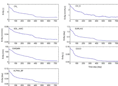
Along with the updating of model states and diagnostic variables, the model parameters are also estimated. Figure 4 shows examples of real-time parameter updating from the ASS_D scenario. After about 130 time steps, the ensemble trajectories are nearly stable with slow variations which are probably induced by the changes of land surface and river channel conditions for runoff generation and routing (Liu et al., 2008; Troch et al., 2013). At every time step in data as-similation, the parameter samples can be approximated with Gaussian distributions and they are constrained within the prior ranges (Min–Max, see Table 1) as shown in the his-tograms in Fig. 4. This property is favourable for parameter estimation with ensemble-based data assimilation. The un-certainties of parameter estimates at every time step are rep-resented using the ensemble spread (EnSp), which is com-puted based on sample variances (see the illustration in cap-tion of Fig. 5). At the beginning of the data assimilacap-tion, the parameters have broad ensemble spreads. The spreads quickly shrink after 100 time steps with the evolution of the streamflow assimilation, and remain stable after 400 time steps. Therefore, the estimate uncertainties of the parameters decrease with the data assimilation and state updating. More-over, the relative stabilities of ensemble trajectories (Fig. 4) and the ensemble spreads (Fig. 5) imply an attractive poten-tial that it is possible to use short-term data to retrieve optimal estimates of parameters.

Even though the three scenarios provide different param-eter estimates due to the assimilation of different observa-tions, encouraging properties of parameter estimations are achieved in the three scenarios. It is not sure so far whether the parameter estimates converge to their appropriate values in this real-word application, so the parameter estimates re-quire a further validation to evaluate the effectiveness of the PU_EnKF scheme.

3.5 Validation for parameter estimates

Figure 4. Estimations of two typical parameters (CN2and CH_K) from the ASS_D scenario. The histograms in each plot, fitted with the Gaussian distribution function, represent the ensemble distribution at three time steps.

Figure 5. Ensemble spreads (EnSp) of the seven parameters listed in Table 1: EnSp= q

1 Nu

PNu

Figure 6. Streamflow predictions using four scenarios of different parameter sets. Only results of Gauges C and D are shown.

validate parameters of a conceptual hydrological model. For simplicity and consistency, the three single-run predictions are named ASS_D, ASS_BD and ASS_AB, although they are neither assimilation-based predictions nor ensemble pre-dictions. Moreover, the control-run prediction is used for comparison. All four scenarios are run for the period 1 January–31 October 2006. The uncertainties in the input forcing and the model structure are not considered in these predictions.

Figure 6 shows the streamflow prediction errors from the four scenarios. Only the results of Gauges C and D are shown because they are located at the downstream locations in the Zhanghe River basin. The three scenarios using prescribed parameters with estimates from data assimilation achieve better predictions for the two gauges than the control-run scenario. The RMSE of Gauge D from the ASS_D scenario decreases from 5.550 m3s−1to 2.324 m3s−1. Moreover, the ASS_BD scenario provides the best predictions among the four scenarios. All of these improvements are attributable to the appropriate parameter estimates from the data assim-ilation. The ASS_BD scenario renders the most reasonable parameter estimates. Comparably, the parameter estimates from ASS_D are also satisfactory for streamflow predictions, while the estimates from the ASS_AB scenario lead to slight improvements for streamflow predictions. Therefore, the pa-rameter estimation performance of the three scenarios is con-sistent with the prediction of diagnostic variables (i.e. the water discharge) as illustrated in Sect. 3.4. The assimilated

observations from downstream, especially the outlet of the basin, have more important roles than those from upstream for parameter estimation and streamflow predictions in un-gauged subbasins.

4 Conclusions

We present an application of PU_EnKF for improving streamflow predictions at ungauged locations. This scheme features real-time updating and simultaneous state-parameter estimation, considering modelling and observing uncertain-ties. Moreover, the scheme constrains the predictions by the physical rainfall-runoff processes that are defined in the dis-tributed hydrological model (i.e. the SWAT model), and it ac-counts for the correlations of states and parameters between gauged and ungauged subbasins. The correlations are repre-sented by the covariance matrix in the Kalman gain. With the constraint and the correlation representation, the observed in-formation is successfully transferred to ungauged locations and thereby improves streamflow prediction.

(especially the data from the outlet) have important roles to reflect the runoff generation for the entire basin. This data assimilation scheme provides reasonable estimates of model parameters for all computational units (i.e. subbasins and HRUs), including both gauged and ungauged sites, as validated by the conventional single-run simulation. Moreover, the parameter estimates approach nearly stable levels after a small number of time steps (130 steps in this study). The parameter estimates show slow variations to trace parameter travels, which indicates the PU_EnKF has a potential advantage of identifying the changes in underlying land surface (e.g., the land use and land cover changes).

Although favourable performance to improve streamflow predictions is obtained using the EnKF-based scheme, the runoff routing is neglected within the PU_EnKF assimilation set-up because the travel time of generated runoff is less than 1 day in the Zhanghe River watershed. In fact, the time lag of runoff routing is an important factor for short-time (e.g. the hourly step) flood forecasting (Li et al., 2013; Pan and Wood, 2013). Moreover, this scheme is intent on PUB for the nested basins in which the correlations of states and parameters be-tween neighbouring subbasins can be constructed. For sepa-rate basins in the same climatic regions and land surface con-ditions, assimilating other sources of data (e.g. the remotely sensed soil moisture and bright temperature) is expected to improve the predictions of hydrological variables (Troch et al., 2003). Nevertheless, this study provides an encourag-ing application for PUB by assimilatencourag-ing streamflow, which is generally regarded as quality observations compared with the remotely sensed data. There are optional methods to ad-dress PUB, e.g. the Particle-DREAM by Vrugt et al. (2013). It will be an encouraging attempt to compare these methods with distributed hydrological models for hydrological diag-nosis and predictions.

Acknowledgements. We would like to thank Giuliano Di

Bal-dassarre and three anonymous reviewers for their constructive comments to polish this paper. Jasper A. Vrugt provided useful suggestions to improve this study. This work was supported by grants from the National Natural Science Foundation of China (41471019, 51009001), the National High Technology Research and Development Program of China (2013AA122801), and the In-ternational S&T Cooperation Program of China (2012DFG21710).

Edited by: G. Di Baldassarre

References

Ajami, N. K., Duan, Q., and Sorooshian, S.: An integrated hy-drologic Bayesian multimodel combination framework: Con-fronting input, parameter, and model structural uncertainty in hydrologic prediction, Water Resour. Res., 43, W01403, doi:10.1029/2005wr004745, 2007.

Arnold, J. G. and Fohrer, N.: SWAT2000: current capabilities and research opportunities in applied watershed modelling, Hydrol. Process., 19, 563–572, 2005.

Arnold, J. G., Srinivasan, R., Muttiah, R. S., and Williams, J.: Large area hydrologic modeling and assessment part I: Model develop-ment1, JAWRA J. Am. Water Resour. As., 34, 73–89, 1998. Blöschl, G., Reszler, C., and Komma, J.: A spatially distributed flash

flood forecasting model, Environ. Model. Softw., 23, 464–478, doi:10.1016/j.envsoft.2007.06.010, 2008.

Cai, X. L.: Strategy analysis on integrated irrigation water manage-ment with RS/GIS and hydrological model, Ph.D thesis, Wuhan University (China), 2007.

Chen, F., Crow, W. T., Starks, P. J., and Moriasi, D. N.: Improv-ing hydrologic predictions of a catchment model via assimila-tion of surface soil moisture, Adv. Water Resour., 34, 526–536, doi:10.1016/j.advwatres.2011.01.011, 2011.

Clark, M. P., Rupp, D. E., Woods, R. A., Zheng, X., Ibbitt, R. P., Slater, A. G., Schmidt, J., and Uddstrom, M. J.: Hy-drological data assimilation with the ensemble Kalman fil-ter: Use of streamflow observations to update states in a dis-tributed hydrological model, Adv. Water Resour., 31, 1309– 1324, doi:10.1016/j.advwatres.2008.06.005, 2008.

Crow, W. T. and Reichle, R. H.: Comparison of adaptive filtering techniques for land surface data assimilation, Water Resour. Res., 44, W08423, doi:10.1029/2008wr006883, 2008.

Crow, W. T. and Van Loon, E.: Impact of incorrect model error as-sumptions on the sequential assimilation of remotely sensed sur-face soil moisture, J. Hydrometeorol., 7, 421–432, 2006. DeChant, C. M. and Moradkhani, H.: Examining the effectiveness

and robustness of sequential data assimilation methods for quan-tification of uncertainty in hydrologic forecasting, Water Resour. Res., 48, W04518, doi:10.1029/2011wr011011, 2012.

Duan, Q. Y., Sorooshian, S., and Gupta, V.: Effective and efficient global optimization for conceptual rainfall-runoff models, Water Resour. Res., 28, 1015–1031, 1992.

Duan, Q. Y., Sorooshian, S., and Gupta, V. K.: Optimal Use of the Sce-Ua Global Optimization Method for Calibrating Watershed Models, J. Hydrol., 158, 265–284, 1994.

Evensen, G.: Sequential data assimilation with a nonlinear quasi-geostrophic model using Monte Carlo methods to fore-cast error statistics, J. Geophys. Res., 99, 10143–10162, doi:10.1029/94jc00572, 1994.

Evensen, G.: The ensemble Kalman filter: Theoretical formula-tion and practical implementaformula-tion, Ocean. Dynam., 53, 343–367, 2003.

Evensen, G.: Data Assimilation: the Ensemble Kalman Filter, Springer Verlag, Berlin, Heidelberg, 2009.

Gassman, P., Reyes, M., Green, C., and Arnold, J.: The soil and water assessment tool: historical development, applications, and future research directions, Trans. ASABE, 50, 1211–1250, 2007. Gupta, H. V., Clark, M. P., Vrugt, J. A., Abramowitz, G., and Ye, M.: Towards a comprehensive assessment of model structural adequacy, Water Resour. Res., 48, W08301, doi:10.1029/2011wr011044, 2012.

Helton, J. and Davis, F.: Latin hypercube sampling and the propa-gation of uncertainty in analyses of complex systems, Reliabil. Eng. Syst. Safe., 81, 23–69, 2003.

to-wards the river in SWAT, Phys. Chem. Earth, Parts A/B/C, 30, 518–526, doi:10.1016/j.pce.2005.07.006, 2005.

Hrachowitz, M., Savenije, H. H. G., Blöschl, G., McDonnell, J. J., Sivapalan, M., Pomeroy, J. W., Arheimer, B., Blume, T., Clark, M. P., Ehret, U., Fenicia, F., Freer, J. E., Gelfan, A., Gupta, H. V., Hughes, D. A., Hut, R. W., Montanari, A., Pande, S., Tetzlaff, D., Troch, P. A., Uhlenbrook, S., Wagener, T., Winsemius, H. C., Woods, R. A., Zehe, E., and Cudennec, C.: A decade of Predic-tions in Ungauged Basins (PUB) – a review, Hydrolog. Sci. J., 58, 1198–1255, doi:10.1080/02626667.2013.803183, 2013. Lee, H., Seo, D.-J., Liu, Y., Koren, V., McKee, P., and Corby,

R.: Variational assimilation of streamflow into operational distributed hydrologic models: effect of spatiotemporal scale of adjustment, Hydrol. Earth Syst. Sci., 16, 2233–2251, doi:10.5194/hess-16-2233-2012, 2012.

Li, Y., Ryu, D., Western, A. W., and Wang, Q. J.: Assimilation of stream discharge for flood forecasting: The benefits of account-ing for routaccount-ing time lags, Water Resour. Res., 49, 1887–1900, doi:10.1002/wrcr.20169, 2013.

Liu, F.: Bayesian time series: analysis methods using simulation-based computation Ph.D thesis, Institutes of Statistics and Deci-sion Science, Duke University, Durham, North Carolina, USA, 2000.

Liu, Y. and Gupta, H. V.: Uncertainty in hydrologic modeling: To-ward an integrated data assimilation framework, Water Resour. Res., 43, W07401, doi:10.1029/2006WR005756, 2007. Liu, G., Chen, Y., and Zhang, D.: Investigation of flow and transport

processes at the MADE site using ensemble Kalman filter, Adv. Water Resour., 31, 975–986, 2008.

McMillan, H. K., Hreinsson, E. Ö., Clark, M. P., Singh, S. K., Za-mmit, C., and Uddstrom, M. J.: Operational hydrological data assimilation with the recursive ensemble Kalman filter, Hydrol. Earth Syst. Sci., 17, 21–38, doi:10.5194/hess-17-21-2013, 2013. Merz, R. and Blöschl, G.: Regionalisation of catch-ment model parameters, J. Hydrol., 287, 95–123, doi:10.1016/j.jhydrol.2003.09.028, 2004.

Moradkhani, H., Hsu, K.-L., Gupta, H., and Sorooshian, S.: Uncer-tainty assessment of hydrologic model states and parameters: Se-quential data assimilation using the particle filter, Water Resour. Res., 41, W05012, doi:10.1029/2004wr003604, 2005a. Moradkhani, H., Sorooshian, S., Gupta, H. V., and Houser, P.

R.: Dual state-parameter estimation of hydrological models us-ing ensemble Kalman filter, Adv. Water Resour., 28, 135–147, 2005b.

Muleta, M. K. and Nicklow, J. W.: Sensitivity and un-certainty analysis coupled with automatic calibration for a distributed watershed model, J. Hydrol., 306, 127–145, doi:10.1016/j.jhydrol.2004.09.005, 2005.

Neitsch, S., Arnold, J., Kiniry, J., Williams, J., and King, K.: Soil and water assessment tool theoretical documentation version 2000, Grassland, Soil and Water Research Laboratory, Temple, Texas, 2001.

Norbiato, D., Borga, M., Degli Esposti, S., Gaume, E., and An-quetin, S.: Flash flood warning based on rainfall thresholds and soil moisture conditions: An assessment for gauged and un-gauged basins, J. Hydrol., 362, 274–290, 2008.

Pan, M. and Wood, E. F.: Inverse streamflow routing, Hydrol. Earth Syst. Sci., 17, 4577–4588, doi:10.5194/hess-17-4577-2013, 2013.

Parajka, J., Viglione, A., Rogger, M., Salinas, J. L., Sivapalan, M., and Blöschl, G.: Comparative assessment of predictions in ungauged basins – Part 1: Runoff-hydrograph studies, Hy-drol. Earth Syst. Sci., 17, 1783–1795, doi:10.5194/hess-17-1783-2013, 2013.

Ponce, V., Hawkins, R., Golding, B., Smith, R., and Willeke, G.: Runoff curve number: Has it reached maturity?, J. Hydrol. Eng., 1, 11–19, 1996.

Post, D. A. and Jakeman, A. J.: Predicting the daily streamflow of ungauged catchments in SE Australia by regionalising the parameters of a lumped conceptual rainfall-runoff model, Ecol. Model., 123, 91–104, 1999.

Rakovec, O., Weerts, A. H., Hazenberg, P., Torfs, P. J. J. F., and Uijlenhoet, R.: State updating of a distributed hydrological model with Ensemble Kalman Filtering: effects of updating fre-quency and observation network density on forecast accuracy, Hydrol. Earth Syst. Sci., 16, 3435–3449, doi:10.5194/hess-16-3435-2012, 2012.

Rallison, R. and Miller, N.: Past, present and future SCS runoff pro-cedure, in: Rainfall Runoff Relationship, edited by: Singh, V. P., Water Resour. Publ., Littleton, Colo., USA, 353–364, 1981. Reichle, R., McLaughlin, D., and Entekhabi, D.: Hydrologic data

assimilation with the ensemble Kalman filter, Mon. Weather Rev., 130, 103–114, 2002.

Reichle, R. H., Crow, W. T., and Keppenne, C. L.: An adaptive en-semble Kalman filter for soil moisture data assimilation, Water Resour. Res., 44, W03423, 10.1029/2007wr006357, 2008. Sellami, H., La Jeunesse, I., Benabdallah, S., Baghdadi, N.,

and Vanclooster, M.: Uncertainty analysis in model parame-ters regionalization: a case study involving the SWAT model in Mediterranean catchments (Southern France), Hydrol. Earth Syst. Sci., 18, 2393–2413, doi:10.5194/hess-18-2393-2014, 2014.

Sivapalan, M.: Prediction in ungauged basins: a grand challenge for theoretical hydrology, Hydrol. Process., 17, 3163–3170, doi:10.1002/hyp.5155, 2003.

Sivapalan, M., Takeuchi, K., Franks, S. W., Gupta, V. K., Karam-biri, H., Lakshmi, V., Liang, X., McDonnell, J. J., Mendiondo, E. M., O’Connell, P. E., Oki, T., Pomeroy, J. W., Schertzer, D., Uhlenbrook, S., and Zehe, E.: IAHS Decade on Predictions in Ungauged Basins (PUB), 2003–2012: Shaping an exciting fu-ture for the hydrological sciences, Hydrolog. Sci. J., 48, 857– 880, doi:10.1623/hysj.48.6.857.51421, 2003.

Srinivasan, R., Zhang, X., and Arnold, J.: SWAT ungauged: hydro-logical budget and crop yield predictions in the Upper Missis-sippi River Basin, Trans. ASABE, 53, 1533–1546, 2010. Tran, A. P., Vanclooster, M., Zupanski, M., and Lambot, S.: Joint

estimation of soil moisture profile and hydraulic parameters by ground-penetrating radar data assimilation with maximum likelihood ensemble filter, Water Resour. Res., 50, 3131–3146, 10.1002/2013WR014583, 2014.

Troch, P. A., Paniconi, C., and McLaughlin, D.: Catchment-scale hydrological modeling and data assimilation, Adv. Water Re-sour., 26, 131–135, doi:10.1016/s0309-1708(02)00087-8, 2003. Troch, P. A., Carrillo, G., Sivapalan, M., Wagener, T., and

van Griensven, A., Meixner, T., Grunwald, S., Bishop, T., Diluzio, M., and Srinivasan, R.: A global sensitivity analysis tool for the parameters of multi-variable catchment models, J. Hydrol., 324, 10–23, doi:10.1016/j.jhydrol.2005.09.008, 2006.

Vrugt, J. A., Diks, C. G. H., Gupta, H. V., Bouten, W., and Verstraten, J. M.: Improved treatment of uncertainty in hydro-logic modeling: Combining the strengths of global optimiza-tion and data assimilaoptimiza-tion, Water Resour. Res., 41, W01017, doi:10.1029/2004wr003059, 2005.

Vrugt, J. A., ter Braak, C. J. F., Clark, M. P., Hyman, J. M., and Robinson, B. A.: Treatment of input uncertainty in hy-drologic modeling: Doing hydrology backward with Markov chain Monte Carlo simulation, Water Resour. Res., 44, W00b09, doi:10.1029/2007wr006720, 2008.

Vrugt, J. A., ter Braak, C. J., Diks, C. G., and Schoups, G.: Hydro-logic data assimilation using particle Markov chain Monte Carlo simulation: Theory, concepts and applications, Adv. Water Re-sour., 51, 457–478, 2013.

Wang, D., Chen, Y., and Cai, X.: State and parameter estimation of hydrologic models using the constrained ensemble Kalman filter, Water Resour. Res., 45, W11416, doi:10.1029/2008wr007401, 2009.

Xie, X.: Simult aneous State-Parameter Estimation for Hydro-logic Modeling Using Ensemble Kalman Filter. Land Sur-face Observation, Modeling and Data Assimilation, 441–464, doi:10.1142/9789814472616_0014, 2013.

Xie, X. and Cui, Y.: Development and test of SWAT for modeling hydrological processes in irrigation districts with paddy rice, J. Hydrol., 396, 61–71, doi:10.1016/j.jhydrol.2010.10.032, 2011. Xie, X. and Zhang, D.: Data assimilation for distributed

hydrolog-ical catchment modeling via ensemble Kalman filter, Adv. Wa-ter Resour., 33, 678–690, doi:10.1016/j.advwatres.2010.03.012, 2010.

Xie, X. and Zhang, D.: A partitioned update scheme for state-parameter estimation of distributed hydrologic models based on the ensemble Kalman filte, Water Resour. Res., 49, 7350–7365, doi:10.1002/2012WR012853, 2013.

Yang, J., Gong, P., Fu, R., Zhang, M., Chen, J., Liang, S., Xu, B., Shi, J., and Dickinson, R.: The role of satellite remote sens-ing in climate change studies, Nat. Clim. Change, 3, 875–883, doi:10.1038/nclimate1908, 2013.