Technical Note: Initial assessment of a multi method approach to spring flood forecasting in Sweden

www.hydrol-earth-syst-sci.net/20/659/2016/ doi:10.5194/hess-20-659-2016

© Author(s) 2016. CC Attribution 3.0 License.

Technical Note: Initial assessment of a multi-method

approach to spring-flood forecasting in Sweden

J. Olsson1, C. B. Uvo2, K. Foster1,2, and W. Yang1

1_{Research & Development (hydrology), Swedish Meteorological and Hydrological Institute, 601 76 Norrköping, Sweden} 2_{Department of Water Resources Engineering, Lund University, Box 118, 221 00 Lund, Sweden}

Correspondence to: J. Olsson ([email protected])

Received: 18 May 2015 – Published in Hydrol. Earth Syst. Sci. Discuss.: 23 June 2015 Revised: 25 November 2015 – Accepted: 12 January 2016 – Published: 10 February 2016

Abstract. Hydropower is a major energy source in Sweden, and proper reservoir management prior to the spring-flood onset is crucial for optimal production. This requires accurate forecasts of the accumulated discharge in the spring-flood pe-riod (i.e. the spring-flood volume, SFV). Today’s SFV fore-casts are generated using a model-based climatological en-semble approach, where time series of precipitation and tem-perature from historical years are used to force a calibrated and initialized set-up of the HBV model. In this study, a num-ber of new approaches to spring-flood forecasting that reflect the latest developments with respect to analysis and mod-elling on seasonal timescales are presented and evaluated. Three main approaches, represented by specific methods, are evaluated in SFV hindcasts for the Swedish river Vindeläl-ven over a 10-year period with lead times between 0 and 4 months. In the first approach, historically analogue years with respect to the climate in the period preceding the spring flood are identified and used to compose a reduced ensemble. In the second, seasonal meteorological ensemble forecasts are used to drive the HBV model over the spring-flood pe-riod. In the third approach, statistical relationships between SFV and the large-sale atmospheric circulation are used to build forecast models. None of the new approaches consis-tently outperform the climatological ensemble approach, but for early forecasts improvements of up to 25 % are found. This potential is reasonably well realized in a multi-method system, which over all forecast dates reduced the error in SFV by ∼4 %. This improvement is limited but potentially significant for e.g. energy trading.

1 Introduction

In Sweden, seasonal (or long-term) hydrological forecasts are used primarily by the hydropower industry for dam reg-ulation and production planning (e.g. Arheimer et al., 2011). The forecasts may be used to optimize the balance between a sufficiently large water volume for optimal power production and a sufficient remaining capacity to safely handle sudden inflows. In northern Sweden, the spring-flood forecast is the most important seasonal hydrological forecast and it gener-ally covers the main snowmelt period in May, June and July. Traditionally, discharge and spring-flood forecasting at seasonal timescales have been based on two approaches. The first utilizes statistical relationships between accumu-lated discharge during the forecasting period and predictors such as snow water equivalent and accumulated precipita-tion that represent the hydrological state at the forecast date (e.g. Garen, 1992; Pagano et al., 2009). The other approach is based on a hydrological model, which is initialized with observed data up to the forecast issue date and then forced with historical meteorological inputs over the forecasting pe-riod (e.g. Day, 1985; Franz et al., 2003). In addition, hybrid approaches, applying model-derived information in the sta-tistical regression, have been proposed (e.g. Nilsson et al., 2006; Rosenberg et al., 2011).

scientific basis of such predictions is that the sea surface temperature (SST), which characteristically evolves slowly, drives the predictable part of the climate. Consequently, pro-viding to a GCM the information about the variations in SST makes possible the forecast of seasonal climate. The SST in-formation may be provided to the GCM by using the SST field as a boundary condition or by coupling the GCM to an ocean model that will then provide the necessary SST infor-mation. GCM seasonal forecasts may be downscaled dynam-ically (e.g. Graham et al., 2007; Bastola et al. 2013; Bastola and Misra, 2014) or statistically (e.g. Uvo and Graham, 1998; Landman et al., 2001; Nilsson et al., 2008), to better repre-sent regional interests.

An early attempt to use climate model output for hydrolog-ical forecasting in a coastal Californian basin during winter 1997/1998 was made by Kim et al. (2000). They found an overall decent agreement between simulated and observed discharge. Low (high) flows were however systematically overestimated (underestimated), which was attributed pri-marily to climate model precipitation bias. To tackle this problem of climate model biases, Wood et al. (2002) pro-posed bias correction by a percentile-based mapping of the climate model output to the climatological distributions of the input variables. Recently, several investigations have fo-cused on the relative role of uncertainties in the initial state and in the climate forecast, respectively, for the hydrological forecast skill (e.g. Li et al., 2009; Shukla and Lettenmaier, 2011).

In a climate-based statistical approach, connections be-tween climate phenomena that affect the large-scale atmo-spheric circulation and the subsequent hydro-meteorological development in specific locations are identified and uti-lized (e.g. Jónsdótir and Uvo, 2009). Such connections are known as teleconnections as they link phenomena occur-ring in widely separated regions of the world. The impacts of the El Niño–Southern Oscillation on the tropical climate are the most commonly used of such teleconnections in sea-sonal forecast (Troccoli, 2010). Teleconnections can be also the basis for seasonal forecast in high latitudes such as the impacts of the North Atlantic Oscillation in the winter cli-mate in Scandinavia (e.g. Uvo, 2003) and the more recently identified impacts of the Scandinavian pattern on summer cli-mate in southern Sweden (Engström, 2011; Foster and Uvo, 2012). Teleconnection indices have also been used as predic-tors in regression-based approaches to seasonal hydrological forecasting (e.g. Robertson and Wang, 2012).

In light of the above-described progress of the field, it is time to explore ways of updating operational practices by in-corporating the new knowledge acquired and methods devel-oped. The objective of this study has been to develop, test and evaluate new approaches to spring-flood forecasting in Sweden. The current spring-flood forecasting practice at the Swedish Meteorological and Hydrological Institute (SMHI) is an example of the traditional model-based approach. It is a climatological ensemble approach based on the HBV

hydro-logical model (e.g. Bergström, 1976; Lindström et al., 1997). The main scientific hypothesis examined is that the applica-tion of large-scale climate data (historical and forecasted) can improve forecast skill, as compared with today’s procedure. A secondary hypothesis is that a combination of approaches provides an added value, as compared with each individual approach. Three different approaches have been tested and evaluated: (1) identification of analogue historical years that resemble the weather in the current year, (2) use of meteo-rological seasonal forecasts as input to the HBV model and (3) application of statistical relationships between large-scale circulation variables and spring-flood volume. The new ap-proaches were evaluated for the spring-flood forecasts 2000– 2010 issued in January, March and May for the river Vin-delälven in Sweden.

2 Material

2.1 Study area, local data and models

The catchment of the river Vindelälven has been used for testing spring-flood forecast. Vindelälven is unregulated and two stations were selected for evaluation of the forecast methods: Sorsele located in the upstream part of the basin and Vindeln at basin outlet (Fig. 1a). The catchment’s el-evation range is ∼260–840 m a.s.l. and ∼5 % of the area consists of lakes. The annual mean temperature is−0.7◦C and precipitation∼780 mm. Figure 2a shows the mean an-nual hydrograph for station Vindeln (1981–2010), which is the period of interest in this study. In January–February the temperature is generally below−10◦C and very little runoff is generated. Melting generally starts in late April, and the subsequent spring flood extends throughout July, followed by elevated discharge levels also in August–October.

In this study we focus on forecasts of the accumulated dis-charge in the spring-flood period (May–July), which is the key variable delivered to the hydropower industry. This quan-tity will in the following be referred to as SFV (spring-flood volume). The mean SFV at station Vindeln (Table 1), corre-sponds to an average discharge in the spring-flood period of ∼380 m3s−1. SFV has a pronounced inter-annual variabil-ity, which is illustrated by its range (Table 1) and frequency distribution (Fig. 2b).

The HBV model (Bergström, 1976; Lindström et al., 1997) was set up and calibrated for Vindelälven, divided into 18 subcatchments with a mean size of 740 km2. HBV is a rainfall-runoff model which includes conceptual numerical descriptions of hydrological processes at basin scale. The general water balance in the HBV model can be expressed as

P−E−R= d

dt[SP+SM+UZ+LZ+VL], (1)

where P denotes precipitation, E evapotranspiration,

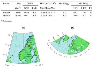
up-Table 1. Basin and station characteristics including overall performance of the HBV model. MARE (%) of SFV estimated by simula-tion (SIM) and by climatological ensemble (CE) forecasts (F) with different issue dates (1/1, 1/3, 1/5). All values represent 2000–2010.

Station Area HBV SFV (m3×109) MARESIM MARECE

(km2) NSE RVE Min/Mean/Max F 1/1 F 1/3 F 1/5

Sorsele 6054 0.89 3.2 1.61/2.30/2.77 6.8 19.2 11.6 9.5 Vindeln∗ 11 846 0.91 1.5 2.26/3.18/4.11 8.2 20.0 13.2 9.0 ∗_{Basin outlet}

Figure 1. Domain used in the CP method, ECMWF IFS grid (blue dots), Vindelälven catchment (yellow), stations Sorsele (S) and Vin-deln (V) (a). Domain used in the SD method (b).

Figure 2. Mean annualQ cycle (a) and SFV frequency distribu-tion (b) for stadistribu-tion Vindeln in the period 1961–1999.

per and lower groundwater, respectively, and VL the volume of lakes. Input data are normally daily observations of P, air temperatureT and monthly estimates of potential evapo-transpiration; output is daily Q. Temperature data are used for calculations of snow accumulation and melt and pos-sibly potential evaporation. The model consists of subrou-tines for meteorological interpolation, snow accumulation and melt, evapotranspiration estimation, a soil moisture ac-counting procedure, routines for runoff generation and, fi-nally, a simple routing procedure between subbasins and lakes. Applying the model necessitates calibration of a num-ber of free parameters, generally about 10.

For historical simulation and calibration, dailyP andT in-puts for the Vindelälven basin were aggregated to basin scale from gridded fields (4×4 km2), created by optimal interpo-lation with altitude and wind taken into account (e.g. Johans-son, 2002). These data, as well asQobservations, are avail-able from 1961. The HBV set-up used in this experiment is the continuously updated and re-calibrated version used operationally, conceivably representing the optimal perfor-mance currently attainable. The calibration is mainly based on the historical period prior to the evaluation period (1961– 1999), but some re-calibration has been done also later.

The overall accuracy of the HBV calibration expressed in terms of the Nash–Sutcliffe efficiency (NSE) and the relative volume error (RVE) in period October 1999–September 2010 are given in Table 1. Values of NSE∼0.9 and only a few percent volume error imply an accurately calibrated model with limited scope for improvement.

2.2 Large-scale atmospheric data

and east Atlantic pattern were collected from the Climate Prediction Center (Climate Prediction Center, 2015).

The atmospheric seasonal forecast data used in this work were obtained from the European Centre for Medium-Range Weather Forecasts (ECMWF). Two model combinations were available: the ECMWF IFS (Integrated Forecast Sys-tem, version 3) coupled with a 1◦version of the HOPE ocean model and the ARPEGE atmospheric model coupled with the variable-resolution (0.33–2◦) ORCA ocean model. Atmo-spheric seasonal forecasts were used in two different forms: seasonal averages from both IFS and Arpege were used in the statistical downscaling Sect. 3.1), and daily time series from IFS were used in the dynamical modelling (Sect. 3.1).

– Seasonal averages: these data are the ensemble means of the different predicted fields covering the domain 75◦W to 75◦E and 80 to 20◦N with a 2◦×2◦ reso-lution. The predicted fields considered were 2 m T, 10 m meridional wind velocity, meridional wind stress, 10 m zonal wind velocity, zonal wind stress, surface sensi-ble heat flux, surface latent heat flux, total precipitation, 850 hPa T, 850 hPa specific humidity, 850 hPa merid-ional wind velocity, 850 hPa zonal wind velocity and 850 hPa geopotential height. The number of ensemble members per field is 11 for the period 1982–2006 (IFS) or 1982–2007 (Arpege) and 41 for the remaining years until 2010. The domain is shown in Fig. 1a.

– Daily time series: these data are the forecasted daily values of 2 m T and the accumulated totalP from the forecast issue date to the forecasting period. These data spanned a period from 2000 to 2010 and had a domain covering 11 to 23◦E and 55 to 70◦N with a 1◦×1◦ res-olution. Figure 1a shows this 1◦×1◦grid in relation to Sweden.

3 Experimental set-up

Three new approaches to seasonal hydrological forecasting are presented and compared to the current climatological semble procedure currently applied at SMHI: analogue en-semble, dynamical modelling and statistical downscaling. All methods are described in detail in the Supplement; be-low only brief outlines are given.

Figure 3 shows a schematic of the “temporal set-up” of the experiments. A key issue in seasonal forecasting is the lead time (green area in Fig. 3), i.e. the period between the fore-cast issue date and the start of the forefore-casting period (blue area). It may be expected that the relative skill of the differ-ent approaches depends on the lead time. Generally, the main gain of statistical approaches is expected for long lead times. When approaching the forecasting period, the representation of the hydro-meteorological state in the HBV model becomes gradually more important, and the relative skill of the cur-rent procedure is likely to increase. To assess the relative

Figure 3. Temporal set-up of the experiments. Vertical black lines: forecast dates. Blue area: spring-flood period. Green area: lead time. Red area: full historical period used in the selection of analogue years (CP, TCI). Black arrows: time periods (1–6 months back in time) tested in the selection of analogue years (CP, TCI). Yellow ar-rows: time period (3 months ahead) used to calculate the predictors in the SD method. White arrows: forecasting periods in which the HBV model was run using full historical ensemble (CE), reduced analogue ensemble (CP, TCI) and ECMWF forecasts (DM).

skill for different lead times, we evaluate historical forecasts (re-forecasts) issued on 1 January (1/1), 1 March (1/3) and 1 May (1/5) in the period 2000–2010.

3.1 Methods

– Climatological ensemble (CE): in this procedure, HBV is initialized by driving it with observed meteorological inputs (P andT) for a spin-up period up to the forecast issue date. Then, all available historical dailyP andT

series in the period from the forecast issue date to the end of the forecasting period are used as input to HBV, generating an ensemble of spring-flood forecasts. For more details, see Supplement, Sect. S1.

– Analogue ensemble (AE): the hypothesis is that it is possible to identify a reduced set of historical years (an analogue ensemble) that describes the weather in the coming forecasting period better than the full histor-ical ensemble used in CE. Two methods for identify-ing analogue years are used, both based on analyses of large-scale atmospheric conditions 1–6 months prior to the forecast issue date (Fig. 3): (1) teleconnection in-dices (TCI) – evolution of inin-dices representing different climate phenomena – and (2) circulation patterns (CPs) – frequencies of weather types that describe the large-scale atmospheric state. The analogue ensemble is then used in the same way as the full ensemble in the CE method. For more details, see Supplement, Sect. S2. – Dynamical modelling (DM): HBV is initialized as in the

CE method. ThenT andP from meteorological sea-sonal forecasts (Sect. 2.2) are converted to HBV input and used to drive the model in the forecasting period. For more details, see Supplement, Sect. S3.

3.2 Evaluation

As described in the Supplement, all methods generate en-semble forecasts (although the AE approach may become deterministic if only one analogue year is found). The en-semble size, however, varies between methods as well as be-tween years for the same method (Supplement, Table S1). Although probabilistic forecasts are generally more useful than deterministic ones, for this initial assessment, with only an 11-year evaluation period, we consider it sufficient with a deterministic evaluation. Thus, from all ensemble forecasts the median forecast is calculated and used in the subsequent analysis, neglecting any impact of ensemble size on the skill of the median (e.g. Buizza and Palmer, 1998).

Forecast performance is assessed by MAREF, the mean absolute value of the relative error of a certain forecast (or simulation) F, defined as

MAREF= 1 11

2010 X

y=2000

AREy_F, (2)

where y denotes year and AREy_F the absolute value of the relative error

AREy_F=

100· SFV

y

F−SFV

y

OBS SFVy_OBS

!

, (3)

where OBS denotes observation.

To quantify the gain of the new forecast approaches (Sects. 3.2–3.4), their MARE values are compared with the MARE obtained using the current CE procedure (MARECE) by calculating the relative improvement, RI (%), according to

RIF=100·

_MARE

CE−MAREF MARECE

, (4)

where a positive RI indicates that the error of the new ap-proach is smaller than the error in the CE procedure and vice versa, and RI=100 % implies a perfect forecast.

As an additional performance measure, we use the fre-quency of years FY+ (%) in which the new approach per-forms better (i.e. has a lower ARE) than the CE procedure. This may be expressed as

FY+_F =100· 1 11

2010 X

y=2000 Hy

!

, (5)

whereHis the Heaviside function defined by

Hy= (

0,AEy_CE < AEy_F 1,AEy_CE > AEy_F

. (6)

As expected considering the short 11-year evaluation period, MARE is sensitive to single years with a high ARE value.

As shown in the results below (Sect. 4), in several cases this makes RI negative even if the new approach outperforms CE in most years (i.e. FY+_{>50). Thus, in this study we}

con-sider FY+to be the most relevant measure of forecast per-formance, although in practice this should be determined to-gether with end-users of the forecasts, based on e.g. the im-pacts of very inaccurate forecasts.

3.3 Baseline simulations with climatological ensemble (CE)

Before testing the new forecasting approaches, the perfor-mance of HBV model and the climatological ensemble pro-cedure (CE) was assessed (Table 1). In simulation mode, i.e. using the actually observed values ofP andT in each year, the MARE of SFV is 7–8 %. This quantifies the HBV model error and corresponds to having a perfect meteorologi-cal forecast. In CE forecast mode, i.e. usingP andT from all historical years as input and to calculate the median SFV, the average MARE decreases gradually from∼20 % in the 1/1 forecasts to∼9 % in the 1/5 forecasts, which thus quantifies the improvement when approaching the spring-flood period. The differences in Table 1 between MARE for simulations and CE forecasts, respectively, represent the part of the total error that is related to the meteorological input. In Vindeläl-ven, this part decreases from 12.1 percentage points in the 1/1 forecasts (which corresponds to∼60 % of the total er-ror) to 1.8 points in the 1/5 forecasts (∼20 %). The relative impact of the HBV model error thus increases with decreas-ing lead time, which implies that the scope for improvdecreas-ing the baseline forecasts decreases with decreasing lead time. It should be emphasized that two out of the three new forecast approaches tested here (AE and DM) aim at improving the meteorological input. They can thus only improve the fore-casts in that respect; the HBV model error remains. The third method (SD), however, aims at improving total performance.

4 Results from single methods

An overview of the results of each approach is given in Ta-ble 2. The numbers after approaches TCI and CP correspond to the best performing version of each approach.

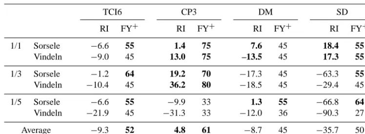
Table 2. Relative improvement RI (%) and frequency of years with a better performance FY+(%) of the new forecasting approaches TCI6, CP3, DM and SD, as compared with the climatological ensemble CE (boldface indicates better performance than CE).

TCI6 CP3 DM SD

RI FY+ RI FY+ RI FY+ RI FY+ 1/1 Sorsele −6.6 55 1.4 75 7.6 45 18.4 55

Vindeln −9.0 45 13.0 75 –13.5 45 17.3 55

1/3 Sorsele −1.2 64 19.2 70 −17.3 45 −63.3 55 Vindeln −10.4 45 36.2 80 −18.5 45 −29.4 45

1/5 Sorsele −6.6 55 −9.9 33 1.3 55 −66.8 64 Vindeln −21.9 45 −31.3 33 −12.0 36 −90.3 27

Average −9.3 52 4.8 61 −8.7 45 −35.7 50

the 1/1 forecasts,N=6 was clearly superior but for the later forecastsN=1 andN=2 produced a similar performance.

The CP method turned out to be more successful, and the resulting SFV forecasts on 1/1 and 1/3 for the best perform-ing version (N=3; CP3) clearly outperformed CE in both stations (Table 2). SFV was more accurately forecasted than with CE in 3/4 of all years. For the 1/5 forecasts, however, CP was less accurate than CE. For the 1/1 and 1/3 forecasts,

N=3 was clearly superior, but for the 1/5 forecastsN=2 andN=4 performed slightly better.

Overall, the DM approach of using ECMWF seasonal forecasts of T andP as inputs to the HBV model did not improve performance as compared with the CE procedure (Table 2). In total, a similar performance to CE was found in station Sorsele, but the accuracy in station Vindeln was consistently lower. In the 1/5 forecasts, however, DM is the overall best performing new approach.

The SD method outperformed CE in the 1/1 forecasts with an RI of almost 20 % in both stations (Table 2). For the 1/3 and 1/5 forecasts the SD method has FY+_{values>50 in}

sta-tion Sorsele but RI values of∼ −65 %. This implies that the SD forecast is generally better than CE but that it may also be very wrong.

The performance of the SD method is heavily affected by whether the climatic features in the forecasting data were en-countered in the training period data set. If the forecasted conditions are outside the range encountered in the training period, the SD method has the tendency to produce forecasts that differ drastically from the observations. This can be dealt with either by increasing the length of the training data set or by analysing the year in question and determining if there were similar years in the training period which would give an indication as to how the method might perform.

With very few exceptions, the new approaches performed better in the upper part of the catchment (Sorsele) than in the outlet (Vindeln). This has not been analysed in any depth, but it is likely related to the more clear-cut spring flood in the upper part with very little prior runoff. In the outlet,

melt-ing episodes before the sprmelt-ing-flood onset lead to temporary increased runoff and a reduction of the snow pack. These episodes, and their impacts, are likely very difficult to cap-ture in seasonal forecasts.

5 Composing a multi-method system

A multi-method forecast approach consists in combining forecasts resulting from different methods to reach a more reliable estimate of the forecast probability distribution. This technique has been used since early 1990s for developing seasonal climate forecast (Tracton and Kalnay, 1993) and has proved to provide more skilful results than a simple model forecast (Hagedorn et al., 2005; among many others).

There are many possible ways of combining or merg-ing multi-method forecasts, rangmerg-ing from simple rank-based methods to more sophisticated statistical concepts. In light of the limited material available in this study, we restricted our-selves to testing two conceptually straightforward ways of combining the forecasts: a median approach (Sect. 5.1) and a weighted approach (Sect. 5.2). Further, the value of using transparent and easily communicated approaches should not be underestimated when the target is operational forecasting and its associated end-user interaction.

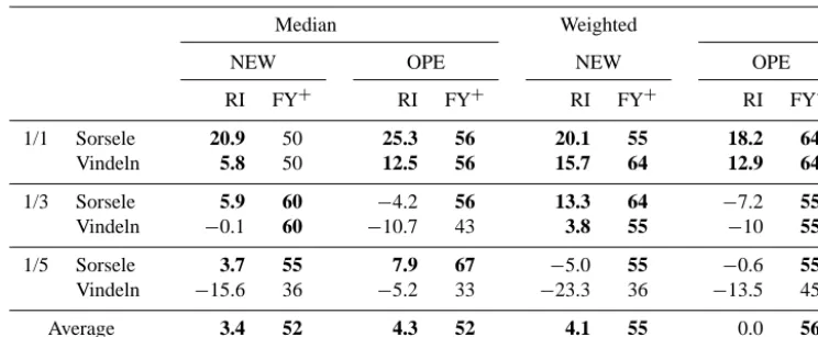
Table 3. Relative improvement RI (%) and frequency of years with a better performance FY+(%) for the median and weighted multi-method approaches, as compared with the climatological ensemble CE (boldface indicates better performance than CE).

Median Weighted

NEW OPE NEW OPE

RI FY+ RI FY+ RI FY+ RI FY+ 1/1 Sorsele 20.9 50 25.3 56 20.1 55 18.2 64

Vindeln 5.8 50 12.5 56 15.7 64 12.9 64

1/3 Sorsele 5.9 60 −4.2 56 13.3 64 −7.2 55 Vindeln −0.1 60 −10.7 43 3.8 55 −10 55

1/5 Sorsele 3.7 55 7.9 67 −5.0 55 −0.6 55 Vindeln −15.6 36 −5.2 33 −23.3 36 −13.5 45

Average 3.4 52 4.3 52 4.1 55 0.0 56

is replaced by CE and thus no attempt to identify analogue years is made here.

5.1 Median multi-method

As three forecasts are available, the median approach amounts to using the second member in the ranked forecast ensemble. For the NEW ensemble, RI indicates a clear im-provement in the 1/1 forecasts as compared with CE, but no improvement in terms of FY+ (Table 3). The 1/3 forecasts are better than CE 60 % of the time, and MARE is slightly reduced on average. The 1/5 forecasts are slightly better than CE in Sorsele but slightly worse in Vindeln. On average, a slight improvement over CE is found. In the OPE ensemble, the 1/1 forecasts perform slightly better than the NEW en-semble but the 1/3 forecasts clearly worse, as expected from the good performance of CP in these forecasts (Table 2). Overall the performance of the OPE ensemble is very sim-ilar to the NEW ensemble (Table 3).

In total, a reduction of MARE by up to 25 % appears at-tainable for the 1/1 forecasts by the median approach. At the later forecast issue dates, a limited improvement in terms of both RI and FY+ was attained for Sorsele but not for Vin-deln. Over all forecast dates and stations, a slight improve-ment over CE is indicated. In some cases, the median multi-method performs slightly better than each of the single meth-ods included, generally because very inaccurate single fore-casts become eliminated.

5.2 Weighted multi-method

This approach consists of applying weights w between 0 and 1 to the different forecasts and then adding them together. The spring-flood volume forecasted by the weighted multi-method, SFVFW, is thus defined as

SFVFW= 3 X

f=1

wf·SFVfwith 3 X

f=1

wf=1 andwf≥0, (7)

where the indexf refers to the three different forecast meth-ods available in each of the ensembles NEW and OPE.

One set of weights is chosen for each forecast date. The selection of weights was made based on the evaluations per-formed in Table 2. With three forecast methods available (in each ensemble), the best performing method (defined by considering both RI and FY+) was assigned the high-est weight 0.5 (=3/6), the second best performing method the intermediate weight 0.33 (2/6) and the worst performing method the lowest weight 0.17 (1/6).

The weighted NEW set outperforms CE in the 1/1 and 1/3 forecasts for both stations; only the 1/5 forecasts for station Vindeln become notably better by CE (Table 3). In the OPE set, similarly to the median forecast, the 1/3 forecast is no-tably worse than the NEW set but still with FY+>50; the 1/5 forecasts are very similar. In total, weighting is not able to improve the result as compared with median approach in terms of RI. However, over all combinations of forecast dates and stations except the 1/5 forecast in station Vindeln, the weighted forecasts perform better than CE in most years (Ta-ble 3). The 1/1 forecasts are better than CE in almost 2/3 of all years with a consistent MARE reduction of 15–20 % in both stations.

6 Concluding remarks

None of the new approaches consistently outperformed the CE method, although improvement was indicated. The largest improvement was found for the 1/1 and 1/3 forecasts using an analogue ensemble based on circulation patterns and for the 1/1 forecasts using statistical downscaling. In these cases the new approach may outperform the CE method up 75 % of the time with an error reduction of ∼20 %. In the 1/5 forecasts, none of the new methods clearly outperformed the CE method. By combining the different methods in a multi-method, an overall slight improvement over CE was attained, with a performance for single forecast dates and sta-tions rather close to the best performing individual method. The overall error reduction attainable by the multi-method, ∼4 %, may sound limited but it must be emphasized that ev-ery percent of forecast improvement potentially corresponds to large financial revenues in energy trading activities. For spring-flood forecasts early in the season, particularly in Jan-uary, the multi-method clearly outperformed the CE method. It must be emphasized that these results were obtained in a preliminary feasibility study with limited data and over-all basic versions of the used methods. Future studies need to include longer test periods and more stations as well as refined and better tailored versions of the forecast methods. One limitation concerns inhomogeneities of data and fore-casts in the study period, e.g. the shift from ERA40 to ERA Interim in 2003 and the shift from 11 to 41 ensemble mem-bers in the seasonal forecasts in 2006/2007. A new ECMWF IFS version (4) is now available, but preliminary tests indi-cate a rather similar performance of SFV forecasts by the approaches concerned, as compared with using the version 3 data as done here. Using bias correction of theP andT in-put in the DM procedure would likely improve performance, as demonstrated by e.g. Wood et al. (2002), although such pre-processing has limitations in an operational context when new model versions are released. Incorporating hydrological model data, in particular snow information, in the SD method has shown promising results in preliminary tests, especially for improving the forecasts close to the spring-flood period. Development and testing along these lines are ongoing.

The Supplement related to this article is available online at doi:10.5194/hess-20-659-2016-supplement.

Author contributions. C. B. Uvo and K. Foster designed and plemented the TCI and SD approaches. W. Yang designed and im-plemented the CP approach. J. Olsson designed and imim-plemented the DM approach and the multi-method composition. J. Olsson pre-pared the manuscript with contributions from mainly C. B. Uvo but also W. Yang and K. Foster.

Acknowledgements. The study was performed in research projects funded by Elforsk AB and the Swedish Research Council Formas. Many thanks to Johan Södling, Jonas German and Barbro Jo-hansson for technical assistance as well as fruitful discussions. Constructive and detailed reviews of the original manuscript by Peter Krahe, Massimiliano Zappa, Renaud Marty and Philippe Cro-chet are gratefully acknowledged.

Edited by: E. Toth

References

Arheimer, B., Lindström, G., and Olsson, J.: A systematic review of sensitivities in the Swedish flood-forecasting system, Atmos. Res., 100, 275–284, 2011.

Bastola, S. and Misra, V.: Evaluation of dynamically downscaled re-analysis precipitation data for hydrological application, Hydrol. Process., 28, 1989–2002, 2014.

Bastola, S., Misra, V., and Li, H. Q.: Seasonal hydrological forecasts for watersheds over the southeastern United States for the boreal summer and fall seasons, Earth Interact., 17, 1–22, 2013. Bergström, S.: Development and application of a conceptual runoff

model for Scandinavian catchments, SMHI Reports RHO No. 7, SMHI, Norrköping, Sweden, 1976.

Buizza, R. and Palmer, T. N.: Impact of ensemble size on ensemble prediction, Mon. Weather Rev., 126, 2503–2518, 1998. Climate Prediction Center: http://www.cpc.ncep.noaa.gov/data/

teledoc/telecontents.shtml, last access: 12 November 2015. Day, G.: Extended streamflow forecasting using NWSRFS, J. Water

Resour. Pl. Manage., 111, 157–170, 1985.

Dee, D. P., Uppala, S. M., Simmons, A. J., Berrisford, P., Poli, P., Kobayashi, S., Andrae, U., Balmaseda, M. A., Balsamo, G., Bauer, P., Bechtold, P., Beljaars, A. C. M., van de Berg, L., Bid-lot, J., Bormann, N., Delsol, C., Dragani, R., Fuentes, M., Geer, A. J., Haimberger, L., Healy, S. B., Hersbach, H., Hólm, E. V., Isaksen, L., Kållberg, P., Köhler, M., Matricardi, M., McNally, A. P., Monge-Sanz, B. M., Morcrette, J.-J., Park, B.-K., Peubey, C., de Rosnay, P., Tavolato, C., Thépaut, J.-N., and Vitart, F.: The ERA-Interim reanalysis: configuration and performance of the data assimilation system, Q. J. Roy. Meteorol. Soc., 137, 553– 597, 2011.

Engström, J.: The effect of Northern Hemisphere teleconnections on the hydropower production in southern Sweden, MSc thesis, Department of Earth and Ecosystem Sciences, Physical Geogra-phy and Ecosystems Analysis, Lund University, Lund, 2011. Foster, K. and Uvo, C. B.: Regionalisation of Swedish hydrology,

XXVII Nordic Hydrology Conference, Oulu, 2012.

Franz, K. J., Hartmann, H. C., Sorooshian, S., and Bales, R.: Verifi-cation of National Weather Service ensemble streamflow predic-tions for water supply forecasting in the Colorado River basin, J. Hydrometeorol., 4, 1105–1118, 2003.

Garen, D.: Improved techniques in regression-based streamflow volume forecasting, J. Water Resour. Pl. Manage., 118, 654–670, 1992.

Graham, L. P., Andreasson, J., and Carlsson, B.: Assessing climate change impacts on hydrology from an ensemble of regional cli-mate models, model scales and linking methods – a case study on the Lule River basin, Climatic Change, 81, 293–307, 2007. Hagedorn, R., Doblas-Reyes, F., and Palmer, T.: The rationale

be-hind the success of multi-model ensembles in seasonal forecast-ing – I. Basic concept, Tellus A, 57, 219–233, 2005.

Johansson, B.: Estimation of areal precipitation for hydrological modelling, PhD thesis, Earth Sciences Centre, Report no. A76, Göteborg University, Göteborg, 2002.

Jónsdóttir, J. F. and Uvo, C.B.: Long term variability in Icelandic hydrological series and its relation to variability in atmospheric circulation over the North Atlantic Ocean, Int. J. Climatol., 29, 1369–1380, 2009.

Kim, J., Miller, N. L., Farrara, J. D., and Hong, S.-Y.: A seasonal precipitation and stream flow hindcast and prediction study in the western United States during the 1997/98 winter season using a dynamic downscaling system, J. Hydrometorol., 1, 311–329, 2000.

Landman, W. A., Mason, S. J., Tyson, P. D., and Tennant, W. J.: Sta-tistical downscaling of GCM simulations to streamflow, J. Hy-drol., 252, 221–236, 2001.

Li, H., Luo, L., Wood, E. F., and Schaake, J.: The role of initial conditions and forcing uncertainties in seasonal hydrologic forecasting, J. Geophys. Res., 114, D04114, doi:10.1029/2008JD010969, 2009.

Lindström, G., Johansson, B., Persson, M., Gardelin, M., and Bergström, S.: Development and test of the distributed HBV-96 hydrological model, J. Hydrol., 201, 272–288, 1997. Nilsson, P., Uvo, C. B., and Berndtsson, R.: Monthly runoff

simu-lation: comparison of a conceptual model, neural networks and a combination of them, J. Hydrol., 321, 344–363, 2006.

Nilsson, P., Uvo, C. B., Landman, W., and Nguye, T. D.: Downscal-ing of GCM forecasts to streamflow over Scandinavia, Hydrol. Res., 39, 17–25, 2008.

Pagano, T. C., Garen, D. C., Perkins, T. R., and Pasteris, P. A.: Daily updating of operational statistical seasonal water supply forecasts for the western U.S., J. Am. Water Resour. As., 45, 767–778, 2009.

Robertson, D. E. and Wang, Q. J.: A Bayesian approach to predictor selection for seasonal streamflow forecasting, J. Hydrometeorol., 13, 155–171, 2012.

Rosenberg, E. A., Wood, A. W., and Steinemann, A. C.: Statisti-cal applications of physiStatisti-cally based hydrologic models to sea-sonal streamflow forecasts, Water Resour. Res., 47, W00H14, doi:10.1029/2010WR010101, 2011.

Shukla, S. and Lettenmaier, D. P.: Seasonal hydrologic predic-tion in the United States: understanding the role of initial hy-drologic conditions and seasonal climate forecast skill, Hy-drol. Earth Syst. Sci., 15, 3529–3538, doi:10.5194/hess-15-3529-2011, 2011.

Tracton, M. S. and Kalnay, E.: Operational ensemble prediction at the National Meteorological Center: practical aspects, Weather Forecast., 8, 379–398, 1993.

Troccoli, A.: Seasonal climate forecasting, Meteorol. Appl., 17, 251–268, 2010.

Uppala, S. M., Kållberg, P. W., Simmons, A. J., Andrae, U., Bech-told, V. D. C., Fiorino, M., Gibson, J. K., Haseler, J., Hernandez, A., Kelly, G. A., Li, X., Onogi, K., Saarinen, S., Sokka, N., Allan, R. P., Andersson, E., Arpe, K., Balmaseda, M. A., Beljaars, A. C. M., Berg, L. V. D., Bidlot, J., Bormann, N., Caires, S., Chevallier, F., Dethof, A., Dragosavac, M., Fisher, M., Fuentes, M., Hage-mann, S., Hólm, E., Hoskins, B. J., Isaksen, L., Janssen, P. A. E. M., Jenne, R., Mcnally, A. P., Mahfouf, J.-F., Morcrette, J.-J., Rayner, N. A., Saunders, R. W., Simon, P., Sterl, A., Trenberth, K. E., Untch, A., Vasiljevic, D., Viterbo, P., and Woollen, J.: The ERA-40 re-analysis, Q. J. Roy. Meteorol. Soc., 131, 2961–3012, 2005.

Uvo, C. B.: Analysis and regionalization of northern European win-ter precipitation based on its relationship with the North Atlantic Oscillation, Int. J. Climatol., 23, 1185–1194, 2003.

Uvo, C. B. and Graham, N.: Seasonal runoff forecast for north-ern South America: a statistical model, Water Resour. Res., 34, 3515–3524, 1998.