Development of streamflow drought severity–duration–frequency curves using the threshold level method

Hydrol. Earth Syst. Sci., 18, 3341–3351, 2014 www.hydrol-earth-syst-sci.net/18/3341/2014/ doi:10.5194/hess-18-3341-2014

© Author(s) 2014. CC Attribution 3.0 License.

Development of streamflow drought severity–duration–frequency

curves using the threshold level method

J. H. Sung1and E.-S. Chung2

1_{Ministry of Land, Infrastructure and Transport, Yeongsan River Flood Control Office, Gwangju, Republic of Korea} 2_{Department of Civil Engineering, Seoul National University of Science & Technology, Seoul, 139-743, Republic of Korea}

Correspondence to: E.-S. Chung ([email protected])

Received: 5 October 2013 – Published in Hydrol. Earth Syst. Sci. Discuss.: 3 December 2013 Revised: 16 July 2014 – Accepted: 22 July 2014 – Published: 3 September 2014

Abstract. This study developed a streamflow drought severity–duration–frequency (SDF) curve that is analogous to the well-known depth–duration–frequency (DDF) curve used for rainfall. Severity was defined as the total water deficit volume to target threshold for a given drought dura-tion. Furthermore, this study compared the SDF curves of four threshold level methods: fixed, monthly, daily, and de-sired yield for water use. The fixed threshold level in this study is the 70th percentile value (Q70) of the flow dura-tion curve (FDC), which is compiled using all available daily streamflows. The monthly threshold level is the monthly varyingQ70values of the monthly FDC. The daily variable threshold isQ70 of the FDC that was obtained from the an-tecedent 365 daily streamflows. The desired-yield threshold that was determined by the central government consists of domestic, industrial, and agricultural water uses and environ-mental in-stream flow. As a result, the durations and sever-ities from the desired-yield threshold level were completely different from those for the fixed, monthly and daily levels. In other words, the desired-yield threshold can identify stream-flow droughts using the total water deficit to the hydrological and socioeconomic targets, whereas the fixed, monthly, and daily streamflow thresholds derive the deficiencies or anoma-lies from the average of the historical streamflow. Based on individual frequency analyses, the SDF curves for four thresholds were developed to quantify the relation among the severities, durations, and frequencies. The SDF curves from the fixed, daily, and monthly thresholds have comparatively short durations because the annual maximum durations vary from 30 to 96 days, whereas those from the desired-yield threshold have much longer durations of up to 270 days. For the additional analysis, the return-period–duration curve was

also derived to quantify the extent of the drought duration. These curves can be an effective tool to identify streamflow droughts using severities, durations, and frequencies.

1 Introduction

The rainfall deficiencies of sufficient magnitude over pro-longed durations and extended areas and the subsequent re-ductions in the streamflow interfere with the normal agricul-tural and economic activities of a region, which decreases agriculture production and affects everyday life. Dracup et al. (1980) defined a drought using the following properties: (1) nature of water deficit (e.g., precipitation, soil moisture, or streamflow); (2) basic time unit of data (e.g., month, sea-son, or year); (3) threshold to distinguish low flows from high flows while considering the mean, median, mode, or any other derived thresholds; and (4) regionalization and/or stan-dardization. Based on these definitions, various indices were proposed over the years to identify drought. Recent stud-ies have focused on such multi-faceted drought characteris-tics using various indices (Palmer, 1965; Rossi et al., 1992; McKee et al., 1993; Byun and Wilhite, 1999; Tsakiris et al., 2007; Pandey et al., 2008a, b, 2010; World Meteorological Organization, 2008; Nalbantis and Tsakiris, 2009; Wang et al., 2011; Tabari et al., 2013; Tsakiris et al., 2013).

reduces crop yields. Precipitation deficits over a prolonged period that reduce streamflow, groundwater, reservoir, and lake levels result in a hydrological drought. If hydrological droughts continue until the supply and demand of numerous economic goods are damaged, a socioeconomic drought oc-curs (Heim Jr., 2002).

Hydrological and socioeconomic droughts are notably dif-ficult to approach. Nalbantis and Tsakiris (2009) defined a hydrological drought as “a significant decrease in the avail-ability of water in all its forms, appearing in the land phase of the hydrological cycle”. These forms are reflected in var-ious hydrological variables such as streamflows, which in-clude snowmelt and spring flow, lake and reservoir stor-age, recharge of aquifers, discharge from aquifers, and base-flow (Nalbantis and Tsakiris, 2009). Therefore, Tsakiris et al. (2013) described that streamflow is the key variable in de-scribing hydrological droughts because it considers the out-puts of surface runoff from the surface water subsystem, sub-surface runoff from the upper and lower unsaturated zones, and baseflow from the groundwater subsystem. Furthermore, streamflow crucially affects the socioeconomic drought for several water supply activities such as hydropower genera-tion, recreagenera-tion, and irrigated agriculture, where crop growth and yield largely depends on the water availability in the stream (Heim Jr., 2002). Hence, hydrological and socioeco-nomic droughts are related to streamflow deficits with respect to hydrologically normal conditions or target water supplies for economic growth and social welfare.

For additional specification, Tallaksen and van Lanen (2004) defined a streamflow drought as a “sus-tained and regionally extensive occurrence of below average water availability”. Thus, threshold level approaches, which define the duration and severity of a drought event while considering the daily, monthly, seasonal, and annual natural runoff variations, are widely applied in drought analyses (Yevjevich, 1967; Sen, 1980; Dracup et al., 1980; Dalezios et al., 2000; Kjeldsen et al., 2000; American Meteorological Society, 1997; Hisdal and Tallaksen, 2003; Wu et al., 2007; Pandey et al., 2008a; Yoo et al., 2008; Tigkas et al., 2012; van Huijgevoort et al., 2012). These approaches provide an analytical interpretation of the expected availability of river flow; a drought occurs when the streamflow falls below the threshold level. This level is frequently considered a certain percentile flow for a specific duration and assumed to be steady during the considered month, season, or year. Therefore, Kjeldsen et al. (2000) applied three variable threshold level methods using seasonal, monthly, and daily streamflows.

There has been a growing need for new planning and de-sign of natural resources and environment based on the afore-mentioned scientific trends. For design purposes, rainfall intensity-duration-frequency (IDF) curves have been used for a long time to synthesize the design storm. Therefore, many studies have integrated drought severity and duration based on the multivariate theory (Bonaccorso et al., 2003; González

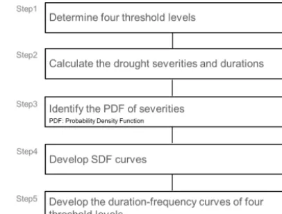
Figure 1. Procedure in this study.

and Valdés, 2003; Mishra and Singh, 2009; Song and Singh, 2010a, b; De Michele et al., 2013). However, these studies cannot fully explain droughts without considering the fre-quency, which resulted in the development of drought iso-severity curves for certain return periods and durations for design purposes.

Thus, based on the typical drought characteristics (wa-ter deficit and duration) and threshold levels, this study de-veloped quantitative relations among drought parameters, namely, severity, duration, and frequency. This study quanti-fied the streamflow drought severity, which is closely related to hydrological and socioeconomic droughts, using fixed, monthly, daily, and desired-yield threshold levels. Further-more, this study proposed a streamflow SDF curve using the traditional frequency analyses. In addition, this study also de-veloped duration frequency curves of four threshold levels from the occurrence probabilities of various duration events using a general frequency analysis because the deficit vol-ume is not sufficient to explain the extreme droughts. This framework was applied to the Seomjin River basin in South Korea.

2 Methodology 2.1 Procedure

J. H. Sung and E.-S. Chung: Development of streamflow drought severity–duration–frequency curves 3343

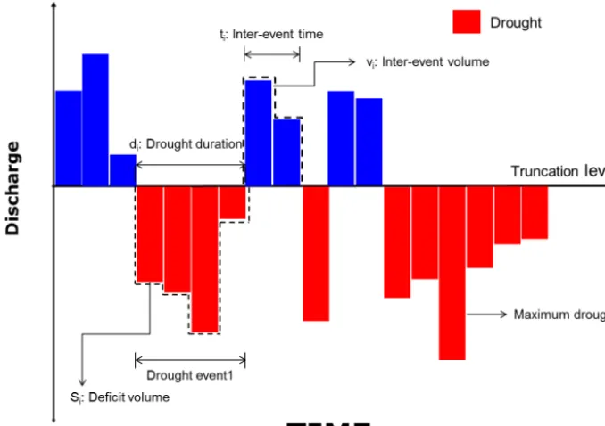
Figure 2. Definition sketch of a general drought event.

descriptions. Step 4 calculates the streamflow drought sever-ities using the selected probability distribution with the best-fit parameters and develops the SDF curves. This step is de-scribed in Sect. 2.5. Step 5 develops the duration–frequency curves of the four threshold levels using an appropriate prob-ability distribution.

2.2 Streamflow drought severity

In temperate regions where the runoff values are typically larger than zero, the most widely used method to esti-mate a hydrological drought is the threshold level approach (Yevjevich, 1967; Fleig et al., 2006; Tallaksen et al., 2009; Van Loon and Van Lanen, 2012). The streamflow drought severity with the threshold level method has the following advantages over the standardized precipitation index (SPI) in meteorology (Yoo et al., 2008) and the Palmer drought sever-ity index (PDSI) in meteorology and agriculture (Dalezios et al., 2000): (1) no a priori knowledge of probability distribu-tions is required, and (2) the drought characteristics such as frequency, duration, and severity are directly determined if the threshold is set using drought-affected sectors.

A sequence of drought events can be obtained using the streamflow and threshold levels. Each drought event is char-acterized by its durationDi, deficit volume (or severity)Si,

and time of occurrenceTi as shown by the definition sketch

in Fig. 2. With a prolonged dry period, the long drought spell is divided into several minor drought events. Because these droughts are mutually dependent, Tallaksen et al. (1997) pro-posed that an independent sequence of drought events must be described using some type of pooling as described below.

If the “inter-event” timeti between two droughts of

du-ration di and di+1 and severity si and si+1, respectively, are less than the predefined critical durationtcand the pre-allowed inter-event excess volumezc, then the mutually de-pendent drought events are pooled to form a drought event as (Zelenhasic and Salvai, 1987; Tallaksen et al., 1997)

dpool =di +di+1+tc

spool =si +si+1−zc. (1)

This study assumedtc=3 days andzc=10 % ofdi ordi+1 for simplicity.

2.3 Threshold selection

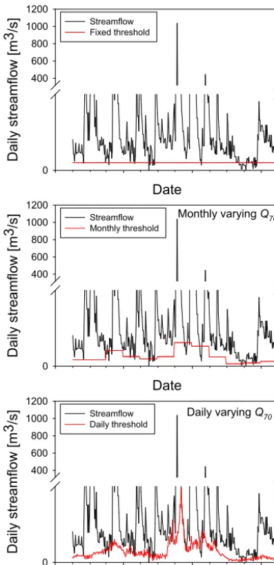
The threshold may be fixed or vary over the course of a year. A threshold is considered fixed if a constant value is used for the entire series and variable if it varies over the year based on the monthly and daily variable levels (Hisdal and Tallaksen, 2003). If the threshold is derived from the flow duration curve (FDC), the entire streamflow record is used in its derivation. As shown in Fig. 3, which is obtained from the study area, fixed and monthly thresholds can be obtained from an FDC and twelve monthly FDCs based on the entire record period. The daily varying threshold can be derived us-ing the antecedent 365-day streamflow.

18

537

538

539

540

Fig. 3. Examples of threshold levels: fixed (top), monthly varying (middle), and daily varying

541 (bottom). 542 543 Date D a ily st re a m fl o w [ m 3/s] 0 400 600 800 1000 1200 Streamflow Fixed threshold Date D a ily st re a m fl o w [ m 3/s] 0 400 600 800 1000 1200 Streamflow Monthly threshold

Monthly varying Q₇₀

Date D a ily st re a m fl o w [ m 3/s] 0 400 600 800 1000 1200 Streamflow Daily threshold

Daily varying Q₇₀

Figure 3. Examples of threshold levels: fixed (top panel), monthly

varying (middle panel), and daily varying (bottom panel).

is the 70th percentile value (Q70) of FDC, which is compiled using all available daily streamflows, and the monthly thresh-old level is the monthly varyingQ70s of each month’s FDC. The daily variable threshold is the Q70 value of the FDC, which is obtained from the antecedent 365 daily streamflows. However, the threshold selection should be further analyzed because it is not clear thatQ70should be used as a represen-tative threshold for rivers in a monsoon climate.

The time resolution, i.e., whether to apply a series of an-nual, monthly, or daily streamflows, depends on the hydro-logic regime in the region of interest. In a temperate zone, a given year may include both severe droughts (seasonal droughts) and months with abundant streamflow, which indi-cates that the annual data do not often reveal severe droughts. Dry regions are more likely to experience droughts that last

for several years, i.e., multi-year droughts, which supports the use of a monthly or annual time step. Hence, different time resolutions may lead to different results regarding the drought event selection. This study used the daily stream-flow data, and various time resolutions (30, 60, 90, 120, 150, 180, 210, 240, and 270 days) were selected to identify the temporal characteristics.

The variable threshold approach is adapted to detect streamflow deviations for both high- and low-flow seasons. Lower than average flows during high-flow seasons may be important for later drought development. However, periods with relatively low flow either during the high-flow sea-son, which can be caused by a delayed onset of a snowmelt flood, are not commonly considered a drought. Therefore, the events that are defined with the varying threshold should be called streamflow deficiencies or streamflow anomalies in-stead of streamflow droughts (Hisdal et al., 2004). In con-trast, the desired yield for sufficient water supply and envi-ronmental in-stream flow can be an effective method to iden-tify a streamflow drought by considering hydrological and socioeconomic demands because environmental in-stream flow has become important in recent years.

2.4 Probability distribution function

An L-moment diagram for various goodness-of-fit tech-niques was used to evaluate the best probability distribu-tion funcdistribu-tion for data sets in several recent studies (Hosking, 1990; Chowdhury et al., 1991; Vogel and Fennessey, 1993; Hosking and Wallis, 1997). The L-moment ratio diagram is a graph where the sample L-moment ratios, L-skewness (τ3), and L-kurtosis (τ4) are plotted as a scatterplot and compared with the theoretical L-moment ratio curves of the candidate distributions. The L-moment ratio diagrams were suggested as a useful graphical tool to discriminate amongst candidate distributions for a data set (Hosking and Wallis, 1997). The sample average and line of best fit were used to select statis-tical distributions, and they can be plotted on the same graph to select the best-fit distribution.

When plotting an L-moment ratio diagram, the relation among the parameters and the L-moment ratiosτ3andτ4for several distributions are required. For a generalized extreme value (GEV) distribution, the three-parameter GEV distribu-tion described by Stedinger et al. (1993) has the following probability density function (PDF,f (x))and cumulative dis-tribution function (CDF,F (x)):

f (x)= 1

α

n 1−κ

α(x−ξ )

o1/κ−1

·exp

−n1− κ

α(x−ξ )

o1/ k

κ 6=0, (2a)

f (x)=1

αexp

−x−ξ

α −exp

−x−ξ

α

κ=0, (2b)

F (x)=exp

−n1− κ

α(x−ξ )

o1/κ

J. H. Sung and E.-S. Chung: Development of streamflow drought severity–duration–frequency curves 3345

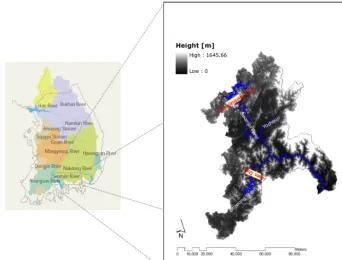
Figure 4. Location of the selected river basin, including elevation and rivers.

F (x) =exp

−exp

−x−ξ

α

κ =0, (3b)

whereξ+α/κ≤x≤ ∞forκ <0,−∞ ≤x≤ ∞for κ=0,

and −∞ ≤x≤ξ+α/κ for κ >0. Here, ξ is a location, α

is a scale, and κ is a shape parameter. Forκ=0, the GEV distribution reduces to the classic Gumbel (EV1) distribution withτ3=0.17. Hosking and Wallis (1997) provided more de-tailed information regarding the GEV distribution. The rela-tion among the parameters andτ3andτ4 for the GEV dis-tribution of the shape parameters can be obtained as follows (Hosking and Wallis, 1997):

τ3=

2 1−3−κ

1−2−κ −3 (4a)

τ4=

5 1−4−κ₋

10 1−3−κ₊

6 1 −2−κ

1−2−κ . (4b)

2.5 Development of the SDF relationships

The IDF or depth–duration–frequency (DDF) curves can be defined to “allow calculation of the average design rainfall intensity (or depth) for a given exceedance probability over a range of durations” (Stedinger et al., 1993). Statistical fre-quency analyses such as rainfall analyses are frequently used for drought events. However, this method cannot fully ex-plain droughts without considering the severity and duration, which resulted in the development of the SDF curve. Thus,

extreme drought events can be specified using the frequency, duration, and either depth or mean intensity (i.e., severity). The frequency is usually described by the return period of the drought. Because its magnitude is given by the total depth that occurs in a particular duration, the SDF relation can be derived. To estimate the return periods of drought events of a particular depth and duration, the frequency distributions can be used (Dalezios et al., 2000).

3 Study region

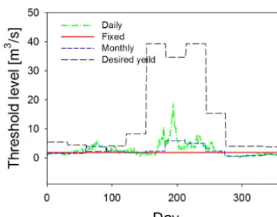
Figure 5. Comparison of the four threshold levels in this study.

water during the dry season (October through March) and flood damage during the wet season.

The administrative districts where the basin is located cover three provinces, four cities, and 11 counties (Nam-won City, Jinan County, Imsil County, and Sunchang County in the northern Jeolla Province; Suncheon City, Gwangyang City, Damyang County, Gokseong County, Gurye County, Hwasun County, Boseong County, and Jangheung County in the southern Jeolla Province; and Hadong County in the southern Gyeongsang Province). The influx rates into the basin from these province are 47 % (southern Jeolla Province), 44 % (northern Jeolla Province), and 9% (south-ern Gyeongsang Province), and a total of 321 104 residents, who occupy 129 322 households, live in these areas.

The land use consists of arable land (876.29 km2), forest land (3400.61 km2), urban area (67.12 km2), and other land uses (567.86 km2). Major droughts occurred in the southern Jeolla Province from 1967 to 1968 and from 1994 to 1995. The Seomjin River basin had <1,000 mm of precipitation on average in 1977, 1988, 1994, and 2008. Among these years, the annual precipitation in 1988 was only 782.7 mm (56.5 %) of the annual average of 1385.5 mm from 1967 to 2008, which represents a severe drought.

4 Results

4.1 Determination of the threshold levels

This study used four threshold levels. The fixed threshold level isQ70 of the FDC, which resulted from 37 year daily streamflows. The monthly thresholds are twelveQ70values of monthly FDCs, which incorporated the data of all daily streamflows from January to December for the past 37 years. The daily threshold isQ70of the FDCs, which resulted from the antecedent 365 daily streamflows. Thus, the daily old level smoothly varies everyday. The desired-yield thresh-old for a sufficient water supply and environmental in-stream flow was determined by the Korean central government. This

Table 1. Monthly average of the four threshold levels.

Threshold level[m3s−1] Fixed Monthly Daily Desired yield

Jan 1.9 1.6 1.5 5.4

Feb 1.9 1.6 2.4 4.5

Mar 1.9 3.9 3.9 2.2

Apr 1.9 2.4 2.5 4.1

May 1.9 1.8 1.9 8.2

Jun 1.9 2.4 3.4 39.4

Jul 1.9 5.9 7.1 34.7

Aug 1.9 5.0 5.1 39.4

Sep 1.9 2.3 2.9 15.4

Oct 1.9 0.6 0.7 4.0

Nov 1.9 0.8 0.9 4.0

Dec 1.9 1.2 1.2 3.8

threshold is related to social and economic droughts because it associates the supply and demand of a number of economic goods and environmental safety. The desired-yield threshold is considerably different from the other levels and represents more realistic conditions because the desired yield is equiva-lent to the planned water supply.

The four calculated thresholds are presented in Fig. 5, and the specific monthly averaged values are listed in Table 1. The average levels were 1.9, 2.5, 2.8, and 13.8 m3s−1for the fixed, monthly, daily and desired-yield levels, respectively. The daily threshold levels, which significantly fluctuated be-cause of the natural streamflow variations during the an-tecedent 365 days, were the largest among the four threshold levels because a summer period (June, July, and August) was considered. The desired-yield level was larger than the fixed, monthly, and daily thresholds. This phenomenon occurred during the winter in Korea, which significantly decreased both the water demand and natural runoff during the win-ter (December, January, and February). However, the thresh-olds for the daily, monthly, and desired-yield levels during the summer were much higher than those during the other seasons. The desired yield during May and June had much higher threshold levels than the other thresholds because this season had the highest agricultural water demand.

4.2 Calculations of the streamflow drought severity and duration

J. H. Sung and E.-S. Chung: Development of streamflow drought severity–duration–frequency curves 3347

21 551

Year

1980 1990 2000 2010

A n n u a l m a x. d ro u g h t d u ra ti o n [ d a y] 0 50 100 150 200 250 Daily Desired yield Fixed Monthly Year

1980 1990 2000 2010

A n n u a l m a x. t o ta l vo lu m e [ m 3 ] 0.0 5.0e+6 1.0e+7 1.5e+7 2.0e+7 2.5e+7 3.0e+7 3.5e+7 Daily Desired yield Fixed Monthly 554

(b) Total water deficit volume (drought severity). 555

Fig. 6. Time series of the annual maxima values of duration and severity. 556

557

(a) Duration.

(b) Severity.

Figure 6. Time series of the annual maxima values of duration and

severity.

water use. Similar to the results for the drought duration, the severities showed much higher values.

To compare the differences among the four threshold lev-els, the correlation coefficients among the water deficits from four different threshold levels were calculated as shown in Table 3. Similar trends were observed for the monthly and daily threshold levels. However, the durations and severities from the desired-yield threshold level were completely dif-ferent from those for the fixed, monthly, and daily levels. In other words, the drought identification techniques based on general threshold levels cannot reflect the socioeconomic drought in terms of the water supply and demand. There-fore, two-way approaches that are categorized using the time periods (fixed, monthly, and daily) for hydrological drought and the desired-yield threshold for socioeconomic droughts should be separately included to identify specific drought characteristics.

4.3 Determination of the probability distribution function

The L-moment diagrams of various goodness-of-fit tech-niques were used to evaluate the best probability distribu-tion funcdistribu-tion for the data sets. To develop a streamflow

Table 2. Summary of the four threshold approaches.

Threshold Maximum Maximum level duration severity

method (days) (m3)

Fixed 92 9 304 762

Monthly 96 10 774 642

Daily 96 18 457 943

Desired yield 232 285 854 400

Table 3. Correlations between the durations and the severities of the

four threshold levels.

Fixed Monthly Daily Desired yield

Duration

Fixed 1

Monthly 0.632 1

Daily 0.632 0.923 1

Desired yield 0.677 0.420 0.475 1

Severity

Fixed 1

Monthly 0.441 1

Daily 0.414 0.853 1

Desired yield 0.281 0.551 0.599 1

drought SDF curve, the proper probability distribution func-tion should be determined based on the statistical results as described in Sect. 2.4.

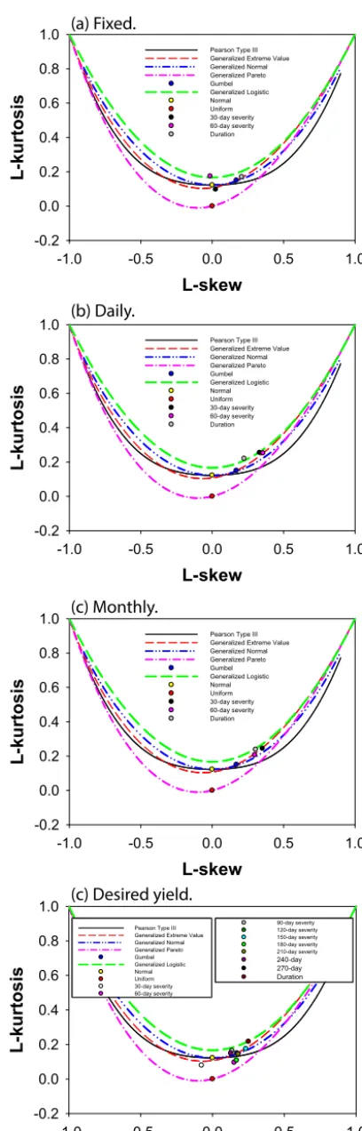
The L-moment ratio diagrams were derived for the four threshold approaches and are shown in Fig. 7. Among the examined distribution models, three parameter distributions (the Pearson Type 3 (PT3), Generalized Normal (GNO), and GEV distributions) appeared consistent with their data sets. In the frequency analysis that addressed extreme values, the distributions that use three parameters were required to ex-press the upper tail. The PT3, GNO, and GEV distributions can be applied in this study. As shown in Fig. 7, this study selected the GEV distribution for a representative probabil-ity distribution because most observations are appropriate for the GEV.

4.4 Development of SDF curves

L-skew

-1.0 -0.5 0.0 0.5 1.0

L-ku rtosis -0.2 0.0 0.2 0.4 0.6 0.8 1.0

Pearson Type III Generalized Extreme Value Generalized Normal Generalized Pareto Gumbel Generalized Logistic Normal Uniform 30-day severity 60-day severity Duration L-skew

-1.0 -0.5 0.0 0.5 1.0

L-ku rtosis -0.2 0.0 0.2 0.4 0.6 0.8 1.0

Pearson Type III Generalized Extreme Value Generalized Normal Generalized Pareto Gumbel Generalized Logistic Normal Uniform 30-day severity 60-day severity Duration L-skew

-1.0 -0.5 0.0 0.5 1.0

L-ku rtosis -0.2 0.0 0.2 0.4 0.6 0.8 1.0

Pearson Type III Generalized Extreme Value Generalized Normal Generalized Pareto Gumbel Generalized Logistic Normal Uniform 30-day severity 60-day severity Duration L-skew

-1.0 -0.5 0.0 0.5 1.0

L-ku rtosis -0.2 0.0 0.2 0.4 0.6 0.8 1.0

Pearson Type III Generalized Extreme Value Generalized Normal Generalized Pareto Gumbel Generalized Logistic Normal Uniform 30-day severity 60-day severity 90-day severity 120-day severity 150-day severity 180-day severity 210-day severity

240-day vs Col 32 270-day vs Col 34 Duration vs Col 36

Pearson Type III Generalized Extreme Value Generalized Normal Generalized Pareto Gumbel Generalized Logistic Normal Uniform 30-day severity 60-day severity 90-day severity 120-day severity 150-day severity 180-day severity 210-day severity

240-day vs Col 32 270-day vs Col 34 Duration vs Col 36 (a) Fixed.

(b) Daily.

(c) Monthly.

(c) Desired yield.

Figure 7. L-moment diagram to identify the probability distribution.

Table 4. Severity–duration–frequency of the desired yield in the

Seomjin River basin.

Duration Return period[yr]

[day] 10 20 50 80 100

30 60.7 66.4 73.1 75.9 77.2

60 82.4 95.9 112.5 120.8 124.9 90 95.6 112.8 133.7 144.6 149.3 120 106.8 132.7 170.0 189.7 200.1 150 116.6 145.2 186.6 208.7 220.3 180 126.0 155.5 197.5 220.8 231.7 210 134.3 168.7 217.7 243.1 257.6 240 141.0 174.2 223.9 248.8 261.3 270 144.6 182.0 233.3 258.9 272.9

100-year frequency. However, the SDF curves from the fixed, daily, and monthly thresholds were calculated using compar-atively short durations because the annual maximum dura-tions vary from 30 to 96 days. Nonetheless, the SDF curve from the desired-yield levels showed the water deficits for much longer durations of 30–270 days. In addition, the wa-ter deficits from the desired-yield levels are much higher than those from other levels even for the same duration.

For a specific description, Table 4 compares all severi-ties to specific frequencies and durations for the desired-yield threshold. When the duration increases, the severity differences among the return periods significantly increase. Therefore, because the streamflow drought severity should be more crucial when the drought continues for a longer pe-riod, the frequency of long droughts should be approached with caution.

4.5 Development of duration–frequency curve

Using the same traditional frequency analysis, the duration– frequency curves for four threshold levels were developed as shown in Fig. 9. In other words, the annual maxima dura-tions are derived based on the four threshold level methods. As shown in the SDF relationship, the GEV distribution was selected from the L-moment ratio diagram. For these plots, 2-, 3-, 5-, 10-, 20-, 30-, 50-, 70-, 80-, and 100-year-frequency severities were calculated. Similar to the SDF curves, the du-rations for the desired-yield threshold were much higher than those for the other three thresholds.

5 Summary and conclusions

J. H. Sung and E.-S. Chung: Development of streamflow drought severity–duration–frequency curves 3349

(a) Fixed. (b) Daily.

(c) Monthly. (d) Desired yield.

Figure 8. SDF curves of the four threshold approaches in the Seomjin River basin.

Figure 9. Duration–frequency curves of the four threshold level

ap-proaches in the Seomjin River basin.

desired-yield levels for water use. In addition, the duration– frequency curves for four thresholds were used to derive the relationship between the drought duration and the drought frequency. This study used the severity, which represents the total water deficit for specific durations. From this study, we can make the following conclusions:

1. The daily threshold levels significantly fluctuated be-cause of the natural streamflow variations for the an-tecedent 365 days and were the largest threshold level because a summer period (June, July, and August) was considered. The desired-yield level was larger than the fixed, monthly, and daily thresholds. This phenomenon occurred during the winter in Korea; thus, both the wa-ter demand and natural runoff during the winwa-ter (De-cember, January, and February) were notably small. 2. The durations and severities from the desired-yield

4. The severities increased with increasing duration and frequency. However, these values were notably different because the four threshold level approaches defined the streamflow drought differently. The SDF curves from the fixed, daily, and monthly thresholds were calculated using comparatively short durations because the annual maximum durations vary from 30 to 96 days. However, the SDF curve from the desired-yield levels shows the water deficits for longer durations of 30–270 days. In addition, the water deficits from the desired-yield levels are significantly higher than those from the others even in the same duration.

5. For the SDF curve of the desired-yield threshold, when the duration increases, the severity differences among return periods significantly increase. Therefore, because the streamflow drought severity should be more cru-cial when the drought continues for a longer period, the frequency of long droughts should be approached with caution.

6. Duration–frequency curves for four threshold levels were also developed to quantify the streamflow drought duration. Similar to the SDF curves, the desired-yield level had much longer durations for the other three thresholds.

7. In the end, the drought identification techniques based on the general threshold levels cannot reflect the socio-economic drought in terms of water supply and demand. Therefore, the two-way approaches that are categorized by the time periods (fixed, monthly, and daily) for hy-drological drought and the desired-yield threshold for socioeconomic drought should be separately included to identify specific drought characteristics.

The streamflow drought SDF curves that were developed in this study can be used to quantify the water deficit for natural streams and reservoirs. In addition, these curves will be extended to allow for regional frequency analyses, which can estimate the streamflow drought severity at ungauged sites. Therefore, they can be an effective tool to identify any streamflow droughts using the severity, duration, and frequency.

Acknowledgements. This study was supported by funding from

the Basic Science Research Program of the National Research Foundation of Korea (2010-0010609).

Edited by: C. De Michele

References

American Meteorological Society: Meteorological drought – Policy statement, B. Am. Meteorol. Soc., 78, 847–849, 1997.

Bonaccorso, B., Cancelliere, A., and Rossi, G.: An analytical for-mulation of return period of drought severity, Stoch. Environ. Res. Risk A., 17, 157–174, 2003.

Byun, H.-R. and Wilhite, D. A.: Objective quantification of drought severity and duration, J. Climate, 12, 747–756, 1999.

Chowdhury, J. U., Stedinger, J. R., and Lu, L.-H.: Goodness-of-fit tests for regional generalized extreme value flood distributions, Water Resour. Res., 27, 1765–1776, 1991.

Dalezios, N., Loukas, A., Vasiliades, L., and Liakopolos, E.: Severity-duration-frequency analysis of droughts and wet peri-ods in Greece, Hydrolog. Sci. J., 45, 751–769, 2000.

De Michele, C., Salvadori, G., Vezzoli, R., and Pecora, S.: Multi-variate assessment of droughts: Frequency analysis and dynamic return period, Water Resour. Res., 49, 6985–6994, 2013. Dracup, J. A., Lee, K. S., and Paulson Jr., E. G.: On the statistical

characteristics of drought events, Water Resour. Res., 16, 289– 296, 1980.

Fleig, A. K., Tallaksen, L. M., Hisdal, H., and Demuth, S.: A global evaluation of streamflow drought characteristics, Hydrol. Earth Syst. Sci., 10, 535–552, doi:10.5194/hess-10-535-2006, 2006. González, J. and Valdés, J. B.: Bivariate drought recurrence

analy-sis using tree ring reconstructions, J. Hydrol. Eng., 8, 247–258, 2003.

Heim Jr., R. R.: A review of twentieth-century drought indices used in the United States, B. Am. Meteorol. Soc., 83, 1149–1165, 2002.

Hisdal, H. and Tallaksen, L. M.: Estimation of regional meteorolog-ical and hydrologmeteorolog-ical drought characteristics: A case study for Denmark, J. Hydrol., 281, 230–247, 2003.

Hisdal, H., Tallaksen, L. M., Clausen, B., and Alan, E. P.: Ch. 5 Hydrological drought characteristics, in: Hydrological Droughts: Processes and Estimation Methods for Streamflow and Ground-water, Developments in Water Science, Elsevier, Amsterdam, 139–198, 2004.

Hosking, J. R. M.: L-moments: Analysis and estimation of distri-butions using linear combinations of order statistics, J. Roy. Stat. Soc. Ser. B, 52, 105–124, 1990.

Hosking, J. R. M. and Wallis, J. R.: Regional Frequency Analy-sis: An Approach Based on L-Moments, Cambridge Univ. Press, New York, 1997.

Kjeldsen, T. R., Lundorf, A., and Dan, R.: Use of two component exponential distribution in partial duration modeling of hydro-logical droughts in Zimbabwean rivers, Hydrolog. Sci. J., 45, 285–298, 2000.

McKee, T. B., Doesken, N. J., and Kleist, J.: The relationship of drought frequency and duration to time scales, Proc. 8th Conf. Appl. Climatol., American Meteor. Soc., Boston, 179–184, 1993. Mishra, A. K. and Singh, V. P.: Analysis of drought sever-ity.area.frequency curves using a general circulation model and scenario uncertainty, J. Geophys. Res., 114, D06120, doi:10.1029/2008JD010986, 2009.

Nalbantis, I. and Tsakiris, G.: Assessment of hydrological drought revisited, Water Resour. Manage., 23, 881–897, 2009.

J. H. Sung and E.-S. Chung: Development of streamflow drought severity–duration–frequency curves 3351

Pandey, R. P., Mishra, S. K., Singh, R., and Ramasastri, K. S.: Streamflow drought severity analysis of Betwa river system (IN-DIA), Water Resour. Manage., 22, 1127–1141, 2008a.

Pandey, R. P., Sharma, K. D., Mishra, S. K., Singh, R., and Galkate, R. V.: Assessing streamflow drought severity using ephemeral streamflow data, Int. J. Ecol. Econ. Stat., 11, 77–89, 2008b. Pandey, R. P., Pandey, A., Galkate, R. V., Byun, H.-R., and Mal, B.

C.: Integrating hydro-meteorological and physiographic factors for assessment of vulnerability to drought, Water Resour. Man-age., 24, 4199–4217, 2010.

Rossi, G., Benedini, M., Tsakins, G., and Giakoumakis, S.: On re-gional drought estimation and analysis, Water Resour. Manage., 6, 249–277, 1992.

Sen, Z.: Statistical analysis of hydrologic critical droughts, J. Hy-draul. Div.-ASCE, 106, 99–115, 1980.

Song, S. B. and Singh, V. P.: Frequency analysis of droughts using the Plackett copula and parameter estimation by genetic algo-rithm, Stoch. Environ. Res. Risk A., 24, 783–805, 2010a. Song, S. B. and Singh, V. P.: Meta-elliptical copulas for drought

frequency analysis of periodic hydrologic data, Stoch. Environ. Res. Risk A., 24, 425–444, 2010b.

Stedinger, J. R., Vogel, R. M., and Foufoula-Georgiou, E.: Fre-quency Analysis of Extreme Events, in: Chapter 18, Handbook of Hydrology, edited by: Maidment, D., McGraw-Hill, Inc., New York, 1993.

Tabari, H., Nikbakht, J., and Talaee, P. H.: Hydrological drought assessment in Northwestern Iran based on streamflow drought index (SDI), Water Resour. Manage., 27, 137–151, 2013. Tallaksen, L. M. and van Lanen, H. A. J.: Hydrological drought:

processes and estimation methods for streamflow and ground-water, Developments in Water Science, Elsevier Science B. V., Amsterdam, 2004.

Tallaksen, L. M., Madsen, H., and Clusen, B.: On the definition and modeling of streamflow drought duration and deficit volume, Hydrolog. Sci. J., 42, 15–33, 1997.

Tallaksen, L. M., Hisdal, H., and van Lanen, H. A. J.: Space-time modelling of catchment scale drought characteristics, J. Hydrol., 375, 363–372, 2009.

Tigkas, D., Vangelis, H., and Tsakiris, G.: Drought and climatic change impact on streamflow in small watersheds, Sci. Total En-viron., 440, 33–41, 2012.

Tsakiris, G., Pangalou, D., and Vangelis, H.: Regional drought as-sessment based on the Reconnaissance Drought Index (RDI), Water Resour. Manage., 21, 821–833, 2007.

Tsakiris, G., Nalbantis, I., Vangelis, H., Verbeiren, B., Huysmans, M., Tychon, B., Jacquemin, I., Canters, F., Vanderhaegen, S., Engelen, G., Poelmans, L., De Becker, P., and Batelaan, O.: A System-based Paradigm of Drought Analysis for Operational Management, Water Resour. Manage., 27, 5281–5297, 2013. van Huijgevoort, M. H. J., Hazenberg, P., van Lanen, H. A. J., and

Uijlenhoet, R.: A generic method for hydrological drought iden-tification across different climate regions, Hydrol. Earth Syst. Sci., 16, 2437–2451, doi:10.5194/hess-16-2437-2012, 2012. Van Loon, A. F. and Van Lanen, H. A. J.: A process-based

typol-ogy of hydrological drought, Hydrol. Earth Syst. Sci., 16, 1915– 1946, doi:10.5194/hess-16-1915-2012, 2012.

Vogel, R. M. and Fennessey, N. M.: L-moment diagrams should re-place product moment diagrams, Water Resour. Res., 29, 1745– 1752, 1993.

Wang, A., Lettenmaier, D. P., and Sheffield, J.: Soil moisture drought in China, 1950–2006, J. Climate, 24, 3257–3271, 2011. World Meteorological Organization: Manual on Low-flow Esti-mation and Prediction, Operational Hydrology Report No. 50, Geneva, 2008.

Wu, J., Soh, L. K., Samal, A., and Chen, X. H.: Trend analysis of streamflow drought events in Nebraska, Water Resour. Manage., 22, 145–164, 2007.

Yevjevich, V.: An objective approach to definition and investigation of continental hydrological droughts, Hydrology Paper No. 23, Colorado State University, Fort Collins, Colorado, USA, 1967. Yoo, C., Kim, D., Kim, T. W., and Hwang, K. N.: Quantification

of drought using a rectangular pulses Poisson process model, J. Hydrol., 355, 34–48, 2008.