Dynamic group decision making

(1)

& Political Science

Dynamic Group Decision Making

Jan Z´apal

A thesis submitted to the Department of Economics of the London School of Economics & Political Science for the degree of Doctor of

(2)

Herman Melville, Moby Dick

(3)

There are too many people to thank. First and foremost, I would like to

thank Ronny Razin for his advice, encouragement and all the time and attention he has devoted over the years as my supervisor. His help has been

invaluable. My gratitude extends to many others at LSE: Gilat Levy, Balazs Szentes, all the members of the theory group and fellow PhD students.

During my Caltech visit, I have greatly benefited from interaction with

Leeat Yariv, Jean-Laurent Rosenthal and Salvatore Nunnari.

On a more personal level, this thesis would have never seen the light of

day without the continuous support of my family, friends, Katka ˇSpániková, M´ıˇsa Krˇc´ılková and a nudge to do a ‘decent PhD’ from Ondˇrej Schneider.

Chapter specific acknowledgements follow. All the remaining errors are my

own.

Chapter 1: For inspiring discussions I would like to thank Marina Agra-nov, Rabah Amir, Martin Gregor, Gene M. Grossman, Rafael Hortala-Vallve, Roman Horvath, Gilat Levy, Francesco Nava, Salvatore Nunnari,

Gerard Padro i Miquel, Thomas R. Palfrey, Torsten Persson, Jean-Laurent

Rosenthal, Balazs Szentes, Leeat Yariv, and seminar participants at Caltech, LSE, IES FSV UK and the XXI SIEP conference in Pavia, Italy. As this

chapter is based on my job market paper, everyone I have talked to about

the paper during the process deserves credit.

Chapter 2: I would like to thank David Baron, John Duggan and Antoine Loeper for discussions about the research presented in this chapter.

Chapter 3: I would like to thank Roman Horv´ath for his invitation to participate on the project that eventually led to this chapter. With

(4)

my co-authors, we thank Marianna Blix-Grimaldi, Jakob de Haan, Michael Ehrmann, Petra Gerlach-Kristen, Etienne Farvaque, Jan Fil´aˇcek, Tom´aˇs

Holub, Jarek Hurn´ık, Jakub Matˇej˚u, Marek Rozkrut, Marek Rusn´ak,

An-drey Sirchenko and seminar participants at the CESifo conference on central bank communication, the European Public Choice Society annual

confer-ence, the Czech Economic Society biennial conferconfer-ence, the Czech National

Bank and the Eurasia Business and Economics Society conference for help-ful discussions. We are gratehelp-ful to Andrey Sirchenko for sharing with us the

data on the voting record in Poland. This research was supported by Czech National Bank Research Project A3/09. We appreciate the support from

(5)

I certify that the thesis I have presented for examination for the MPhil/PhD degree of the London School of Economics & Political Science is solely my

own work other than where I have clearly indicated that it is the work of

others (in which case the extent of any work carried out jointly by me and any other person is clearly identified in it).

The copyright of this thesis rests with the author. Quotation from it is

permitted, provided that full acknowledgement is made. This thesis may not be reproduced without my prior written consent.

I warrant that this authorization does not, to the best of my belief,

infringe the rights of any third party.

I declare that my thesis consists of 33,940 words.

Statement of conjoint work

I confirm that Chapter 3 was jointly co-authored with Kateˇrina ˇSm´ıdkov´a and Roman Horv´ath and I contributed 33.3% of this work.

(6)

A common theme running throughout the three chapters of this thesis is

dynamic recurring group decision making. The first chapter sets up a model with endogenous status-quo (dynamic bargaining model) in which decision

makers are uncertain about their own future preferences. The main focus of the chapter is on how different bargaining protocols influence equilibrium

decisions. The two protocols considered are i)implicit status-quobargaining protocol in which present period policy serves as the status-quo for the next period and ii) explicit status-quo bargaining protocol in which the current decision involves both current policy and a possibly different status-quo

for the future. The main observation of the chapter is that the former bargaining protocol leads to decisions diverging from the preferences of the

actors involved even in the periods in which their preferences coincide, this

divergence being driven by the concerns to maintain a bargaining position for the future. The latter bargaining protocol, on the other hand, delivers

decisions fully reflecting preferences of the actors involved in the periods

when these coincide, but may lead to decisions reflecting only the proposer’s preferences.

The second chapter shows how to construct equilibria in a class of

dy-namic bargaining models in which players have fixed preferences over all the dimensions of a policy space. The construction applies both to

one-dimensional and multi-one-dimensional policy spaces and delivers equilibria with

simple and intuitive structure. The chapter works out several examples to show i) the multiplicity of equilibria and ii) the non-monotonicity of the

existence of the simple equilibria in the underlying model parameters.

The third paper is a collaborative work with Roman Horv´ath and Kateˇrina ˇ

Sm´ıdkov´a from the Czech National Bank (currently published as a CNB

working paper). The chapter analyses decision making in monetary policy committees, the decision making bodies of central banks. On the empirical

(7)

side, the chapter shows that voting records of monetary policy committees are informative about their own future decisions. On the theoretical side,

the chapter shows that the voting records’ predictive power can be generated

(8)

Introduction 14

1 Explicit and implicit status-quo determination in dynamic

bargaining: Theory and application to FOMC directive 19

1.1 Introduction. . . 20

1.2 Model . . . 27

1.3 Two period model . . . 29

1.4 Infinite horizon model . . . 32

1.5 Re-interpretation of asymmetric FOMC directive . . . 51

1.A1 Proofs . . . 61

1.A2 Static mechanism implementation. . . 108

1.A3 Numerical simulation of equilibrium under explicit status-quo bargaining . . . 109

2 Simple equilibria in dynamic bargaining games over policies115 2.1 Introduction. . . 116

2.2 Literature survey . . . 117

2.3 Model . . . 120

2.4 Equilibria withX ∈R . . . 121

2.5 Equilibria withX ∈Rn . . . 129

2.6 Discussion . . . 134

2.7 Conclusion . . . 136

2.A1 Proofs . . . 137

3 Central Banks’ Voting Records and Future Policy (joint work with Roman Horv´ath and Kateˇrina ˇSm´ıdkov´a)146 3.1 Introduction. . . 147

3.2 Related Literature . . . 149

(9)

3.3 A Model of Central Bank Board Decision-Making . . . 152

3.4 Institutional Background. . . 171

3.5 Empirical Methodology . . . 175

3.6 Empirical Results . . . 179

3.7 Concluding Remarks . . . 189

3.A1 Derivation of Central Bank Board Decision-Making Model and Simulation Robustness Checks . . . 190

3.A2 Data . . . 208

(10)

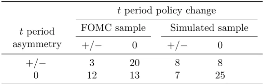
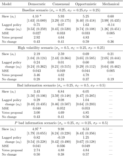
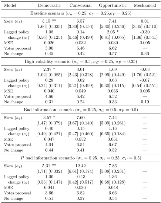
1.1 Predicting future policy changes hypothesis

t+ 1 period policy change and tperiod asymmetry . . . 56

1.2 Consensus building hypothesis

tperiod policy change andt period asymmetry . . . 57

1.3 Authoritarian regime

predicting future policy/consensus building hypothesis . . . . 58

3.1 Does the Voting Record Predict Policy Rate Changes?

Estimates Using Simulated Data with N = 4 and ρ= 0.95

∆pt+1 =a0+a1skewt+a2∆pt+ut+1 . . . 166

∆pt+1 =a0+a1skewt+a2∆pt+ut+1 . . . 167

Estimates Using Simulated Data

∆pt+1 =a0+a1skewt+a2∆pt+ut+1 . . . 170

3.4 Does the Voting Record Predict Repo Rate Changes?

Baseline Estimates

∆it+1=b0+b1skewτ(t)+b2∆it+b3(iχ(t),L−iχ(t),S) +ut+1 . 180

Alternative Specifications - Different Maturities in Term Struc-ture and Uncertainty

∆it+1=b0+b1skewτ(t)+b2∆it+b3(iχ(t),L−iχ(t),S)+b4dispersiont+ ut+1 . . . 183

Alternative Specifications - Data until Financial Crisis Only ∆it+1=b0+b1skewτ(t)+b2∆it+b3(iχ(t),L−iχ(t),S) +ut+1 . 185

(11)

3.7 Does the Voting Record Predict Repo Rate Changes in the USA?

Chappell, McGregor, and Vermilyea (2005) Data for Burns and Greenspan Era

∆it+1=b0+b1skewτ(t)+b2∆it+b3dispersiont+b4committee biast+ ut+1 . . . 187

3.8 Does the Voting Record Predict Repo Rate Changes in the

USA?

Chappell et al. (2005) Data for Burns and Greenspan Era Skew for Alternate Members Added

∆it+1=b0+b1skewτ(t)+b2∆it+b3dispersiont+b4committee biast+ b5skew alternatest+ut+1 . . . 188

∆pt+1 =a0+a1skewt+a2∆pt+ut+1 . . . 200

∆pt+1 =a0+a1skewt+a2∆pt+ut+1 . . . 201

∆pt+1 =a0+a1skewt+a2∆pt+ut+1 . . . 202

∆pt+1 =a0+a1skewt+a2∆pt+ut+1 . . . 203

Estimates Using Simulated Data with N = 4 and ρ1 = 1.95,

ρ2 =−0.98

∆pt+1 =a0+a1skewt+a2∆pt+ut+1 . . . 204

Estimates Using Simulated Data with N = 6 and ρ1 = 1.95,

ρ2 =−0.98

∆pt+1 =a0+a1skewt+a2∆pt+ut+1 . . . 205

3.15 Does the Voting Record Predict Policy Rate Changes? Opportunistic Model with Simple Majority, Estimates Using

Simulated Data with N = 4

(12)

3.16 Does the Voting Record Predict Policy Rate Changes? Opportunistic Model with Simple Majority, Estimates Using

Simulated Data with N = 6

(13)

1.1 Equilibrium policy with implicit status-quo

π∗= 2, φ= 1, δ = 0.5, rd= 0.5 . . . 37

1.2 Equilibrium policy with explicit status-quo

π∗= 2, φ= 1, δ = 0.5, rd= 0.5 . . . 43

1.3 Equilibrium status-quo with explicit status-quo

π∗= 2, φ= 1, δ = 0.5, rd= 0.5 . . . 44

1.4 Long-run status-quo with explicit status-quo

average over 10.000 random 100 period long paths

π∗= 2, φ= 1, δ = 0.5, rd= 0.5 . . . 46

1.5 Equilibrium value functions

π∗= 2, φ= 1, δ = 0.5, rd= 0.5 . . . 48

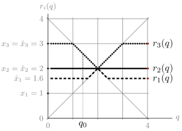
2.1 Conjectured equilibrium in Example 2.1 . . . 123

3.1 Simulated Policy Paths . . . 168

3.2 Actual Voting Record Skew and Future Policy Rate Change . 174

(14)

The common denominator of my thesis is recurrent group decision making.

A group of decision makers is repeatedly making the same type of decision. Once a decision is made in a given bargaining round it determines the

status-quo for the subsequent round. The resulting endogeneity of the status-quo makes the situation one of dynamic bargaining. The rationale for the

explicit modelling of such situations comes from an attempt to understand

the determination of policies that need to be continuously specified over time, such as central bank interest rates, tax rates or regulatory limits.

The dynamic bargaining literature, to which this thesis contributes, grew

from the original bargaining model of Rubinstein (1982) and its political economy application by Baron and Ferejohn (1989). Where the dynamic bargaining literature diverges from these papers is in assuming that reaching

a decision does not end the bargaining process, proceeding into a next period of typically infinite horizon interaction instead. What makes the interaction

dynamic, as opposed to repeated, is the endogeneity of status-quo. A current

decision is made against the status-quo determined by previous decisions and will in turn determine the status-quo in the future. Baron (1996) is among the first to analyse a model with these features.1

In this context, the first chapter focuses on the role of the bargaining protocol in the dynamic bargaining model with uncertainty regarding future

preferences of the actors involved. The chapter compares two bargaining

protocols: i) the implicit status-quo protocol under which present period policy serves as the status-quo for the next period and ii) theexplicit status-quo protocol under which the decision in the current period involves both current policy and a (possibly different) status-quo for the ensuing period. While the former bargaining protocol is standard in the dynamic bargaining

1

See chapter2for survey of the dynamic bargaining literature.

(15)

literature, the latter one and their comparison is the key novel feature. The chapter shows that the two bargaining protocols lead to notably

different policy outcomes, with the difference most marked in the periods

of common interest. These are still characterized by disagreement under implicit status-quo bargaining, while under explicit status-quo bargaining

lead to the policy decisions that fully reflect the congruent preferences of

the committee members. This result arises due to the dual role of policy under the implicit status-quo protocol. Policy serves not only as policy

but also determines the future status-quo and hence the bargaining position of committee members. The disagreement then arises even in periods of

common interest due to the possibility of future conflict. The explicit

status-quo protocol retains only the former role of policy with the policy decisions fully reflecting the common interests, when these arise.

A second difference arising from the two bargaining protocols is in the

evolution of bargaining power as captured by the status-quo. The explicit status-quo protocol allows the proposer, by giving her more flexibility in

crafting her proposals, to gain and retain the dominant position in the

com-mittee. Relative to implicit status-quo bargaining, this results in the policy outcomes that reflect, to a larger extent, the proposer’s preferences, policy

outcomes that are too extreme from the point of view of the committee as

a whole.

The differences in the policy outcomes also determine the answer to

a question on which of the two bargaining protocols would be chosen by a

committee of decision makers who know it would be used in their subsequent interaction, or by a utilitarian central planner. The chapter shows that the

explicit status-quo protocol is superior only if the initial status-quo gives

little bargaining power to the proposer, such that the benefits of the common interests being reflected in the decisions outweigh the costs of the proposer’s

dominance.

The second chapter shows how to construct equilibria in the dynamic bargaining model, with fixed preferences of the players involved and, in the

terminology of the previous chapter, with implicit status-quo bargaining protocol. For a similar model of bargaining over the share of a fixed-size

budget, this has been done byKalandrakis(2004), but for a model based on

Baron (1996) where the bargaining proceeds over a one-dimensional space

(16)

in the dynamic bargaining literature.

The bargaining proceeds over a space of policies with each player having

quadratic preferences defined around a bliss point, where the policy space

can be either one-dimensional as inBaron (1996) or multi-dimensional. In the absence of dynamic considerations the player recognized to be a

pro-poser would propose her bliss point and, given sufficiently adverse

status-quo, would have it approved by at least a minimum winning coalition of the remaining committee members. The chapter shows that in the same

situation, the player recognized to be a proposer proposes herstrategic bliss point, a policy between her and the median player’s original bliss points.

The exact position of the strategic bliss point for a given player depends

on the model parameters, such as the discount factor and the probability of being recognized as a proposer, but is shown to be the result of two

opposing forces. One force pushes the player into proposing policies close

to her original bliss point. The second and strategic force pushes the player in the opposite median player’s direction, in an attempt to propose policies

that constrain the future proposals of all the remaining players.

The chapter constructs an algorithm that calculates the strategic bliss points for a given model parametrization and shows how to use these to build

conjectured equilibrium strategies. It further derives two conditions, one

suf-ficient and one necessary, that the conjectured strategies need to satisfy in order to constitute an equilibrium. Both of these conditions are easy to check

as they consider only a finite set of points in otherwise continuous policy

space. Finally, the chapter works out several examples showing a number of interesting features that equilibria in the model may exhibit. These include

a subset of players behaving in a way indistinguishable from the behaviour

of the median player despite having different preferences, asymmetric equi-librium behaviour in otherwise symmetric environments and multiplicity

of equilibria possibly complicating their computational approximation that

typically relies on the uniqueness of the equilibrium being approximated. The third chapter is an application of the dynamic bargaining framework

to central bank decision making. In most modern central banks decisions to change or retain a given interest rate level is done by a group of decision

makers, the monetary policy committee. The committee meets in a recurring

(17)

status-quo for the next one.

The chapter builds on the observation made by Gerlach-Kristen (2004) for the Bank of England that a voting pattern from a given monetary

pol-icy committee meeting is informative regarding interest rate changes in the subsequent meetings. The chapter finds similar result in voting and

deci-sion making data from several other central banks and, from the theoretical

perspective, asks if it is possible to generate predictive power of the voting pattern in a formal group decision making model.

The model used posits a committee of decision makers making recurring decisions about policy, trying to match an unobserved time-varying optimal

policy that follows AR(1) process. Non-unanimous voting arises from the

committee members having private signals about the optimal policy and hence voting either for the status-quo or for the policy proposed by the

committee chairman. The alternative attracting (super-)majority of votes

then becomes status-quo for the subsequent committee meeting.

The chapter investigates three variants of the model that differ in the

degree of informational influence among the committee members. In the

democraticversion the influence is limited with committee members extract-ing no information from the chairman’s proposal and the chairman havextract-ing

no information regarding signals of the remaining committee members. In

the consensual version it is the chairman who has the informational influ-ence, with the other committee members extracting information from her

proposal, while in theopportunisticversion the influence works in the oppo-site direction, with the chairman having information about private signals of the other committee members.

Using computer simulations, the chapter generates decision making and

voting data from the three model versions and uses these in an econometric estimation akin to the one used with the real world data. The results suggest

that in order to generate predictive power of the voting pattern for the future

policy changes large degree of informational independence is needed, as in the democratic version of the model. The chapter further investigates the

effect of the noise in private signals, of the variability in the optimal policy and of the size of the committee, showing that the size can be used as a

substitute for quality of information in generating predictive power of the

(18)

Baron, D. P. (1996). A dynamic theory of collective goods programs. Amer-ican Political Science Review 90(2), 316–330.

Baron, D. P. and J. A. Ferejohn (1989). Bargaining in legislatures.American Political Science Review 83(4), 1181–1206.

Gerlach-Kristen, P. (2004). Is the MPC’s voting record informative about

future UK monetary policy? Scandinavian Journal of Economics 106(2), 299–313.

Kalandrakis, A. (2004). A three-player dynamic majoritarian bargaining game. Journal of Economic Theory 116(2), 294–322.

Rubinstein, A. (1982). Perfect equilibrium in a bargaining model. Econo-metrica 50(1), 97–109.

(19)

Explicit and implicit status-quo

de-termination in dynamic bargaining:

Theory and application to FOMC

directive

(20)

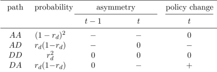
Several other members indicated that they would have preferred to tighten at that meeting. . . . The asymmetric directive, which held prospect of near-term tightening, once again allowed FOMC to reach a consensus.

Meyer(2004), page 83

And we know from firsthand accounts that Greenspan was holding back an FOMC that was eager to raise rates.

Blinder and Reis(2005), page 58

1.1

Introduction

We study recurring group decision making problems with the preferences

of the actors involved varying over time. As a leading example, consider periodic meetings of a monetary policy committee. In every period, the

preferences of each committee member will be affected by host of factors,

such as the state of the economy, his view of future economic development, his opinion about the strength of monetary policy transmission channels,

or judgment about the suitable inflation monetary policy should aim for.

Inevitably, most of those factors will change stochastically over time, opening the possibility for renegotiation of decisions reached at an earlier stage. Of

course, there are many other examples of recurring decision making with

varying preference, both in the economic and the political spheres.

With changing preferences of the involved parties, bargaining over a

decision at any given point in time will proceed under varying degrees of

disagreement. In the monetary policy committee case, ambiguity of infor-mation the committee holds can provoke disagreement over the most

appro-priate policy in some periods, but can lead to agreement in other periods

when the information becomes more definite. Uncertainty over the future then implies uncertainty about the extent of future disagreement as well.

Recurring decisions naturally create dynamic linkages that need to be

considered. First, strategic linkages arise due to the repeated nature of the interaction. The current action of any given decision maker will take into

account its possible impact on the future behaviour of the remaining

(21)

unattainable in static settings. This is analysed in the folk theorems liter-ature in general and in the political arena context in particular by Dixit,

Grossman, and Gul(2000) andMaggi and Morelli(2006). We abstract away

from these strategic linkages in recurring decisions by focusing on Stationary Markov Perfect equilibria.

Instead, we concentrate on the second type of linkages, procedural ones.

These involve the role past decisions play during the determination of sub-sequent ones. These linkages stem from the need to ensure continuity in

policy making. Protocols in place ensure that some policy is chosen even in the case of a decision not being reached.

The simplest of such protocols is the one under which a policy, once

established, becomes the status-quo for the ensuing round of bargaining. Inaction, no change in a given policy or contract, leaves the previous decision

in place. For example, in most countries personal income tax rates apply

until changed. Labour unions negotiate agreements with firms regarding wage and employment levels which are effective until renegotiated. In effect,

current policyimplicitly determines status-quo.

However, there are several prominent examples of decision processes that enlarge the space of current decisions to include provisions for the future.

These yield not only current policy but also explicitly determine a (poten-tially different) status-quo for the next round of negotiations. Legislative

sunset provisionsspecify a time horizon for the statute or regulation in ques-tion, after which it automatically terminates. These are often found in tax

laws or in laws impinging civil liberties, most prominently in the US Eco-nomic Growth and Tax Relief Reconciliation Act of 2001 and US Patriot

Act of 2001. Regulatory escape clauses are another example of the present policy and the status-quo being distinct.1

In this paper, we investigate decisions reached in recurring negotiations

with stochastically changing preferences of the actors involved. The

status-1

(22)

quo for a given round of bargaining is determined endogenously during the previous negotiations. We call the distinction between the new status-quo

being implicitly or explicitly decided uponbargaining protocol and ask how the bargaining protocol influences decisions reached.

We are motivated by normative, positive and theoretical questions. On

the normative side we analyse how the different bargaining protocols

influ-ence the ability of the committee to respond to the changing preferinflu-ences of the involved parties. The procedural linkages mentioned above imply that

the behaviour of each decision maker will reflect both current and future incentives. This might imply that even in ‘agreement’ periods,

character-ized by similar current preferences of the decision makers, their behaviour

might be driven by efforts to affect future decisions. We will show below that enlarging the space of current decisions to include provisions for the

future via the explicit status-quo bargaining protocol delivers policies

bet-ter tailored to changing circumstances. A potential downside of allowing for such provisions comes from the resulting increase in proposal power.

Con-sequently, from the utilitarian perspective none of the bargaining protocols

clearly dominates the other and we lay out conditions under which one or the other of them should be endorsed.

Our positive motivation builds on one of our motivating examples,

mon-etary policy committees. Monmon-etary policy in most central banks is decided upon by a committee composed of several members convening with regular

frequency. The policy usually consists of the bank’s operating target, its

interest rate. In most central banks the interest rate decided in a given committee meeting serves also as a status-quo for the next meeting.

Inac-tion leads to no change in monetary policy stance, hence the status-quo is

implicitly determined by a given decision.

In contrast, the Federal Open Market Committee (FOMC), the decision

body of the US Federal Reserve System, issues at the close of each meeting

operating instructions for the Federal Reserve Bank of New York known as the domestic policy directive. The directive contains not only the decision about current policy but also a statement concerning the FOMC’s expecta-tion of future policy stance. Viewing the ‘asymmetry’, ‘bias’ or ‘tilt’ in the

policy directive as explicitly specifying a status-quo policy possibly different

(23)

decision making process.2 Our model then suggests a novel rationale for the existence of the asymmetry.

The theoretical motivation is to advance growing dynamic bargaining

literature. While acknowledging endogeneity of the status-quo in recurring decision making situations, this literature has invariably assumed that the

status-quo is equal to the policy decision of the previous bargaining round.

While this is a natural assumption in many environments, some environ-ments might be more appropriately modelled as having an explicit

status-quo bargaining protocol. Our analysis of explicit status-status-quo bargaining is not only, to our knowledge, novel in the literature, but also highlights

differ-ences the two bargaining protocols bring by analysing them in an otherwise

identical model setup.

In the model, a committee composed of two members, one of whom

possesses fixed proposal power, takes repeated decisions on a policy from

a one-dimensional policy space over which each of the committee members has single peaked preferences represented by a bliss point. Every period is

randomly selected to be either an agreement or disagreement one, with only

the present period type being common knowledge. In agreement periods, the two members share a common bliss point whereas in the disagreement

periods the bliss points of the two members differ. While certainly a crude

simplification of the continuum on which conflict of preferences can take place, the agreement/disagreement dichotomy allows us to clearly illustrate

the effect of the bargaining protocol on policy outcomes.

Besides the period type, every committee meeting is characterized by a one-dimensional status-quo. Under the implicit status-quo bargaining

pro-tocol, the status-quo is pitched against a proposed policy with the

win-ning alternative being both the current policy outcome and the next period quo. Under the explicit quo bargaining protocol, the

status-quo is pitched against a joint proposal for a policy and a new status-status-quo. If

the committee selects the proposed pair, this proposal determines the cur-rent policy outcome and a possibly diffecur-rent future status-quo, otherwise,

the status-quo becomes both the policy implemented today and the future status-quo.

We first show existence and uniqueness in a certain well defined sense

2

(24)

of Stationary Markov Perfect equilibrium (S-MPE) under both bargaining protocols (propositions1.1 and 1.4). The lack of general S-MPE existence results and typically ill behaved induced preferences over the ‘state’

vari-able in dynamic bargaining models (Baron,1996;Baron and Herron,2003;

Kalandrakis, 2004; Duggan and Kalandrakis, 2012) make this a nontrivial

exercise and we are forced to work with induced preferences that typically

lack monotonicity, concavity and continuity. Adding further stochastic el-ements would allow us to use existing results on existence of S-MPE in

dynamic bargaining context.3 We refrain from doing so, limiting general-ity of our results to cases of sufficiently but not excessively strong conflict

between the two players. On the other hand, this allows us to characterize

equilibria of the model to a greater extent.

For the implicit status-quo bargaining protocol, we show that in

equilib-rium negotiations display inefficiency in agreement periods; the committee

members are unable to agree on a policy corresponding to their common bliss point (proposition 1.2). The intuition for this result is the dual role of policy under the implicit status-quo bargaining protocol. Policy serves

not only as policy but also determines the future status-quo. Moreover, we show that bargaining quickly reaches a point of gridlock, with the

pol-icy outcomes unresponsive to changing preferences (proposition 1.2). Once in gridlock, the two players have antithetic preference over policy even in agreement periods, as it determines the future status-quo and affects their

future bargaining positions. Explicit status-quo bargaining reverses both of

these results. In equilibrium, it leads to the policy outcomes corresponding to the common committee members’ bliss point in the agreement periods

(proposition 1.3) and does not lead to the gridlock as the policy outcomes remain responsive to the changing preferences of the committee members (proposition1.5).

One possible side effect of explicit status-quo bargaining comes from

the increase of proposal power relative to implicit status-quo bargaining. Allowing for proposals with different policy and status-quo creates room

for the proposer to push through policies fully reflecting her preferences. Those are too extreme for the rest of the committee and the committee as a

3

(25)

whole might prefer different bargaining protocols in different environments (proposition1.6).

Finally, we show that these results carry over to a committee composed

of an odd number of members with preferences similar to those in the bench-mark model (proposition1.7). This allows us to shift attention to the FOMC decision making process and examine the role of the asymmetry in its

direc-tive. We focus mainly on its role as a predictor of future policy changes and as an instrument to achieve more consensual FOMC decisions. Our model

delivers these two predictions and also suggests a novel explanation for the existence of the asymmetry as a tool which allows the FOMC chairman to

maintain his dominant position in the committee.

The model we build belongs to the dynamic bargaining literature that assumes that the status-quo during a given round of bargaining is

endoge-nously determined during previous bargaining rounds. Differently from most

of the existing literature (Baron,1996;Baron and Herron,2003;Kalandrakis,

2004;Bernheim, Rangel, and Rayo,2006;Battaglini and Coate,2007;Baron,

Diermeier, and Fong,2012;Battaglini and Palfrey,2012) we focus on an

en-vironment with stochastic preferences and abstract from distributional issues analysed in many of the mentioned papers.

Despite its obvious appeal, the dynamic bargaining literature with

time-varying preferences is rather scarce. Battaglini and Coate (2008) build a dynamic model of legislative bargaining with general and targeted public

spending. In their model, the status-quo is fixed but the intertemporal link

is created by accumulated public debt while the time-varying preferences stem from a stochastic value of general public spending. Diermeier and Fong(2009) build a similar model. Riboni and Ruge-Murcia(2008) analyse a model similar to ours with the implicit status-quo bargaining protocol. They analytically solve the two period version of their model and resort

to numerical simulation of the infinite period version. Dziuda and Loeper (2010) also analyse a model closely related to ours with the implicit status-quo bargaining protocol. In their model, a two member committee takes

repeated decisions over a binary agenda with the preference parameter of each of the committee members being a continuous random variable

dis-tributed on the real line. In our model, it is the preference parameter that

(26)

current decisions to include provisions for the future changes policy out-comes and ability of the committee members to renegotiate in the changing

environment, something our explicit status-quo bargaining protocol does. It

is the comparison between the two bargaining protocols or institutions we are interested in.

Another strand of literature related to this paper is the literature

in-vestigating the effect of linking decisions. In Jackson and Sonnenschein (2007) agents are constrained to represent their preferences across decision problems such that the representation corresponds to the underlying distri-bution of their preferences. The main result of their paper is that linking

large numbers of decisions leads to approximate ex ante Pareto efficiency. In

Casella(2005) agents can store their votes and use them in future meetings

when their preferences are more intense. This typically leads to ex ante

welfare improvement over non-storable votes. Hortala-Vallve (2010) proves similar result in a setting where agents can distribute a given number of votes freely across a predetermined number of issues. The first mentioned

paper improves efficiency by putting constraints on the misrepresentation

of preferences allowed for, while the two latter papers improve efficiency by relaxing the one-person-one-vote constraint. In the context of this

lit-erature, our explicit status-quo bargaining protocol, by relaxing the ‘policy

equal to status-quo’ constraint, can be viewed as relaxing constraint on the committee decision making but also as removing constraint on the proposal

power.

We proceed as follows. The next section lays out the theoretical model. Section 1.3 solves for the equilibrium in a two period version. It is meant to build intuition for the infinite horizon version and to show that the key

results are not sensitive to changes in the foresight horizon. Section 1.4 contains all the theoretical results. These describe equilibria for both of the

bargaining protocols, discuss conditions under which one of them should be

(27)

1.2

Model

We analyse the effect of bargaining protocol on dynamic policy making in

a simple model. Policies in the model are set by a committee composed of two members. The first member is the chairman, who has policy proposal

power and whom we denote byC (she). The second committee member is denoted byP (he) and has policy approval power. The voting rule used by

the committee is simple majority with ties decided againstC’s proposal so

that in order forC’s proposal to pass, consent of both committee members is required.4

The committee sets policyptin each periodtof an infinite horizon. The

utility playeri∈ {C, P}receives from the path of policiesp={p0, p1, p2, . . .}

is given by

Ui(p) = ∞ X

t=0

δtui,t(pt)

whereδ ∈[0,1) is common discount factor. Instantaneous utility ui,t(pt) of

each player is

ui,t(pt) =−(pt−π∗−εi,t)2

where π∗ is a common component in the committee members’ preferences and εi,t is a stochastic time-varyingi−specific preference shock.

The timing of actions in periodt is as follows. First, nature determines

εi,t according to the process specified below and the committee convenes

withxt being the default option. Both εi,t and xt are common knowledge.

Second, the chairmanC proposes a pair γt={pt, qt}against default option

¯

γt ={xt, xt}. Third, voting takes place between γt and ¯γt. If P prefers γt

it is implemented (C always votes for her proposal), players receive their

payoffs from the offered policy pt and the offered status-quo qt becomes

default option for the next period, i.e. xt+1 = qt. If P prefers ¯γt, players

receive their payoffs from the default policy xt and the default status-quo

xt becomes default option for the next period, i.e. xt+1 = xt. Finally, the

committee adjourns and the game moves into periodt+ 1.

In the text we refer to the pair γt = {pt, qt} C proposes as to (C’s) proposal or offer, call its first element pt proposed (offered) policy and its

4 _{An alternative assumption that would not change any of the results is}_C _{making a}

(28)

second element qt proposed (offered) status-quo. The pair ¯γt = {xt, xt}

is then default option or simply default and we abuse notation slightly in calling xt by the same term.

Without loss of generality we assume that C whose utility maximizing offerγtcoincides with the default option ¯γtproposes ¯γtinstead of proposing

a policy she knows would be rejected. It is also easy to see that in any

equilibrium of the game it has to be the case that ifP is indifferent between default ¯γt and C’s proposal γt he votes for γt. As a result C’s offer γt is

always accepted and we do not need to distinguish between proposed and accepted policies.

Up to this point the model generates dynamic policy making in that

the proposed (and hence accepted) status-quo qt from period t becomes

the default option xt+1 for the t+ 1 period. To study how this feature

interacts with the bargaining protocol used by the committee, we contrast

two versions of the model. The first model version and bargaining protocol is with implicit status-quo. Under this bargaining protocol C’s proposals are constrained to those that satisfypt=qtso that the tperiod status-quo

qt, and hencet+ 1 period default optionxt+1, is implicitly defined by thet

period policypt. The second model version and bargaining protocol is with explicit status-quo. Under this bargaining protocol t period status-quo qt,

and hence t+ 1 period default optionxt+1, is explicitly determined during

the committee bargaining.

To close the model we need to specify the distribution of the preference

shocksεi,t. We assume those are generated according to

εi,t= (

−φfori=C and φfori=P with probability rd

0 for i∈ {C, P} with probability 1−rd

whereφ >0 andrd∈[0,1]. In words, there are two types of periods. With

probability rd bliss points in the instantaneous utility functions of C and

P are π∗−φ and π∗+φ respectively. We call those disagreement periods orD periods for short. The second type of period occurs with probability

1−rd and are called agreement periods or A periods for short. In these,

bliss points in the instantaneous utility functions of both players areπ∗. Several comments regarding our modelling choices are in order. First,

(29)

the proposal power to C is motivated by our interest in the trade-off the explicit status-quo bargaining protocol creates. On the one hand, it should

lead to more efficient policy outcomes, but it also opens the door to an abuse

of proposal power. We want to see the full effect on both sides and thus opt for arguably strong assumptions.

Second, having A and D periods in the model reflects our belief that

in recurrent decision making this is a natural assumption. We could have chosen either purely ideological or purely common preferences, which our

model indeed includes as special cases with rd = 1 or rd = 0. However, it

is easy to show that under both specifications the bargaining protocol plays

no role. It is the interaction with the time varying preferences that creates

an interesting problem to study.

1.3

Two period model

To build intuition for the results below, we first solve a two period version of the model. All the results are easily derived using backward induction

and we state them without formal proofs.

Lemma 1.1 (Last period). For the last period default option x1 and both bargaining protocols, equilibrium policy proposals pA,1(x1) and pD,1(x1), in

A and D periods respectively, satisfy

pA,1(x1) =π∗

pD,1(x1) =f(x1, φ)

where f(x, φ) = max{min{2(π∗+φ)−x, x}, π∗−φ}.

In the last period there is no procedural link with the future via the status-quo and hence the bargaining protocol plays no role. It is thus easy

to see why the two policy makers decide on π∗ inA periods as it is a bliss

point in their common utility function.

D period policy then reflects conflict in the committee. P’s acceptance

set consists of a symmetric interval around his bliss point π∗+φwith one

boundary given by default optionx1, [2(π∗+φ)−x1, x1]. C maximizes her

utility with bliss point at π∗−φ by proposing minimum of P’s acceptance

(the min term) but only if she cannot propose her bliss point (the max

(30)

[π∗−φ, π∗+φ], there is no other policy except forx1 the two policy makers

are willing to agree on. P would reject any policy belowx1 andC does not

want to offer any policy abovex1 and thus f(x1, φ) =x1.5

C’s and P’s expected utilities before nature determines the type of last period, as a function of x1 (and hence as a function of the first period

status-quo),

E[UC,0(x1)] =−rd(pD,1(x1)−π∗+φ)2+ (1−rd)·0

E[UP,0(x1)] =−rd(pD,1(x1)−π∗−φ)2+ (1−rd)·0,

reflect intertemporal preferences of the two policy makers and are

inter-esting for several reasons. First, both are non-concave and non-monotone.

E[UC,0(x1)] and E[UP,0(x1)] are non-increasing and non-decreasing

respec-tively for x1 ≤ π∗ +φ and vice-versa for x1 ≥ π∗ +φ. This is the reason

why we cannot work with equilibria associated with well-behaved (concave, monotone) value functions as in, for example, Battaglini and Coate (2007, 2008), as the ill-behaved intertemporal preferences are an inherent feature of the model.

Second, potential future conflict spills over to the current period through

the conflict in the intertemporal preferences. P prefers default optionx1 as

close to π∗+φ as possible while C prefers it as far away from π∗+φ as

possible. Thus the committee members have an incentive to manipulatex1

in the first period as it determines their bargaining positions. Under implicit status-quo bargaining this is done via the enacted policy and under explicit

status-quo bargaining this is done via the enacted status-quo.

Third,E[UC,0(x1)] andE[UP,0(x1)] are constant forx1 ∈/(π∗−φ, π∗+3φ).

For the first period under explicit status-quo bargaining this means that

whenever z /∈ (π∗−φ, π∗+ 3φ) is an equilibrium status-quo proposal for

some default option, so is z0 ∈/ (π∗−φ, π∗+ 3φ). However, this multiplicity has no effect on the last period policy. No matter whether z or z0 is

pro-posed, last periodP’s acceptance set includes, on a policy dimension unique,

unconstrained maximizer of C’s overall utility.

5_{Notice also that the interval where}_f₍_·_,_·_{) is not constant, the interval of default options}

(31)

Lemma 1.2(First period,D). For the first period default optionx0, implicit status-quo protocol policy proposal pI_D,₀(x0) and explicit status-quo protocol policy and status-quo proposalspE_D,₀(x0) and q_D,E₀(x0) in D periods satisfy

pI_D,₀(x0) =pED,0(x0) =qED,0(x0) =f(x0, φ).

For the implicit status-quo protocol this reflects conflict in terms of

both current and intertemporal preferences. The same holds for the ex-plicit status-quo, but C can, in principle, offer a policy different from the

status-quo. To see the nature of her trade-off, C can either concede on the

policy dimension in order to gain a better bargaining position on the status-quo dimension, or vice versa. The strength of those two forces, to satisfy

instantaneous or intertemporal utility, then determines her equilibrium

pro-posal. As we will see below, the two forces exactly cancelling each other, which leads to pE_D,₀(x0) = qD,E0(x0), is a result specific to the two period

model.

Lemma 1.3 (First period, A). For the first period default optionx0, equi-librium policy proposal under the implicit and explicit status-quo protocol,

pI_A,₀(x0) and pEA,0(x0) respectively, in A periods satisfy

pI_A,₀(x0) =f(x0, φκ0)

pE_A,₀(x0) =π∗

where κ0 = δrd

1+δrd ≤

1 2.

First A periods reveal the key difference between the two bargaining

protocols. Under the implicit status-quo bargaining, policy serves two roles.

It is a policy in the standard sense but also determines future bargaining positions. Agreeing on π∗ in A period would entail, at least for one of the

players, giving up bargaining position relative to x0. Combining current

preferences favouring π∗ and intertemporal preferences favouring π∗ −φ

(π∗+φ) for C (P) makes A periods ‘lesser disagreement’ periods with the

degree of conflict given byφκ0. The more probable the true D periods are

and the more players care about future, the more of the conflict spills over toAperiods.

Explicit status-quo bargaining on the other hand implies π∗ is

(32)

policy dimension and, crucially, with the policy and status-quo possibly different, C does not compromise her bargaining position by proposing π∗

policy. To the contrary, this allowsC to propose status-quo that improves

her bargaining position. She has a room to do so since proposingπ∗ on the policy dimension has madeP better off compared to the default option x0.

A key advantage of the two period model just discussed is that it delivers

key predictions about the difference in policy outcomes under the two bar-gaining protocols in a relatively simple framework. On the other hand, with

a fixed time horizon we are unable to discuss the evolution of policies in the long-run, and the fixed horizon also raises concerns about robustness of the

results presented. For this reason we turn to the infinite horizon version of

the model next.

1.4

Infinite horizon model

This section solves the infinite horizon dynamic bargaining model for the two

bargaining protocols. For technical reasons we restrict the proposal space along any dimension to lie in a convex compact subset X of R. Hence for

bothC’s proposals and default options, we haveγt,¯γt∈X2 ⊆R2. However,

it will become apparent from the model equilibria below that withX taken to be ‘sufficiently large’, this assumption is without loss of generality.

We focus on Stationary Markov Perfect Equilibria (S-MPE) where strate-gies in a given period depend only on the type of that period and on the

default option for that period, i.e. only on payoff relevant variables.

Focus-ing on the S-MPE we can drop all time subscripts. We denote byx∈X the default option for a given period with the understanding that it is composed

of a default policy status-quo pair ¯γ(x) ={x, x} ∈X2. Any policy is always denoted by (appropriately subscripted)p∈X and any status-quo is always denoted byq ∈X.

For this model, S-MPE will be a combination of several components. For

C, we are looking for four functions, two of them mapping the space of de-fault optionsXinto proposed policies for each type of period,pD(x), pA(x) :

X2→X, and the remaining two mappingX into the proposed status-quo,

qD(x), qA(x) : X2 → X. Formally, ρC = {pD(x), pA(x), qD(x), qA(x)} :

(33)

i ∈ {A, D} and default option x maps the combination of ¯γ(x) and γi(x)

into his vote, hence it is a mapping ρP :X8 → {yes,no}2.

It has to be acknowledged that our definition ofρC andρP does not allow

for mixed strategies. ForP this is driven by the already mentioned fact that in any equilibrium P’s voting strategy has to be to vote for C’s proposal

γi(x) whenever indifferent betweenγi(x) and ¯γ(x) fori∈ {A, D}. ForCthe

reason behind focusing on pure strategies is twofold. First, we have assumed above thatC whose utility maximizing proposal coincides with the default

option ¯γ(x) indeed proposes ¯γ(x) instead of coming up with a proposal she knows would be rejected. Second, below we focus on a certain class of

equilibria (see definition 1.3) for which it will be true that C’s indifference among K proposals{γ_i1(x), . . . , γ_iK(x)} for some default option x ∈X and

i ∈ {A, D} will imply indifference by P among the same proposals. As a

result, in case ofC’s indifference between two or more proposals we can pick

oneγk_i(x) out of{γ_i1(x), . . . , γ_iK(x)} without changing the equilibrium (via changing the equilibrium value functions defined below) and hence we can

think ofρC as a function instead of thinking of ρC as a distribution onX4.

With this qualification in mind, our definition of S-MPE is as follows.

Definition 1.1(Stationary Markov Perfect Equilibrium). A pair of strate-giesρ∗ ={ρ∗_C, ρ∗_P} constitutes S-MPE if it constitutes subgame perfect equi-librium.

Notice that any given pair of strategies ρ = {ρC, ρP} for given x and

given path of A and D periods generates a unique path of implemented

policies {p0, p1, . . .}. Taking expectations over all possible paths gives a

continuation value function for each policy maker who knows x but does

not know whether the next period will be anA orDone,

V_Cρ(x) =E

"_∞ X

t=0

−δt(pt−π∗+φID(t))2 #

V_Pρ(x) =E

"_∞ X

t=0

−δt(pt−π∗−φID(t))2 #

where ID(t) is D-period indicator function and the superscript ρ captures

(34)

these can be equivalently derived as

V_Cρ(x) =rd

−(pD(x)−π∗+φ)2+δV_Cρ(qD(x))

+ (1−rd)

−(pA(x)−π∗)2+δV_Cρ(qA(x))

V_Pρ(x) =rd

−(pD(x)−π∗−φ)2+δV_Pρ(qD(x))

+ (1−rd)

−(pA(x)−π∗)2+δV_Pρ(qA(x))

.

Finally, we denote by Aρ_i(x) P’s acceptance set in period i ∈ {A, D} given default optionx and strategies ρ. The acceptance sets are given by

Aρ_D(x) ={{p, q} ∈X2| −(p−π∗−φ)2+δV_Pρ(q)≥ −(x−π∗−φ)2+δV_Pρ(x)}

Aρ_A(x) ={{p, q} ∈X2| −(p−π∗)2+δV_Pρ(q)≥ −(x−π∗)2+δV_Pρ(x)}

and both are nonempty as ¯γ(x)∈Ai(x) for i∈ {A, D}.

With this notation, C’s problem can be restated in terms of a pair of

the usual Bellman functional equations

U_Dρ(x) = max

{p,q}∈Aρ_D(x)

{−(p−π∗+φ)2+δrdU_Dρ(q) +δ(1−rd)U_Aρ(q)}

U_Aρ(x) = max

{p,q}∈Aρ_A(x)

{−(p−π∗)2+δrdUDρ(q) +δ(1−rd)UAρ(q)}

(1.1)

where C’s continuation value function V_Cρ will be the probability-weighted sum of the value functions of the two optimization problems, i.e. V_Cρ =

rdUDρ + (1−rd)UAρ. An alternative definition of S-MPE that exploits the

recursive structure of the model and that we use is the following.

Definition 1.2(Stationary Markov Perfect Equilibrium). A pair of strate-gies ρ∗ = {ρ∗_C, ρ∗_P} constitutes a S-MPE if for all x ∈ X and any period

i∈ {A, D}

1. C’s proposal strategy ρ∗_C solves (1.1)

2. P votes for C’s proposal γi(x) if and only if γi(x)∈Aρ

∗

i (x).

An equivalent way to express the requirement of the S-MPE is to say we

are looking for ρ giving rise to V_Cρ and V_Pρ such that when C and P max-imize their utility in the current period, their optimal behaviour is indeed

expressed as ρ. If we can find such a ρ then by the one deviation principle

we have an equilibrium.

Below, when we discuss S-MPE for the two bargaining protocols, it will

become apparent that many of them satisfy an additional restriction in P

(35)

C’s offer, provided C’s proposal differs from the unconstrained maximizer of her overall utility. Another way to view this is that as long as the default

option x providesP with any real bargaining power,C’s proposal will

pro-vide him with the minimum utility sufficient for her proposal to pass. We call S-MPE satisfying this feature Conflict S-MPE (CS-MPE). Denoting by

γ_CDρ and γ_CAρ solutions to the two optimization problems in (1.1) when the restrictions on {p, q} to lie in P’s acceptance sets are removed, CS-MPE is defined as follows.

Definition 1.3 (Conflict Stationary Markov Perfect Equilibrium). A pair of strategies ρ∗ ={ρ∗_C, ρ∗_P} constitutes a CS-MPE if for all x∈X and any periodi∈ {A, D}

1. ρ∗ constitute a S-MPE

2. P is indifferent between γi(x) and γ¯(x) provided γCi∈/ Aρ_i(x).

Our focus on CS-MPE has another rationale as it can be viewed as a

fo-cus on equilibria with the minimum winning coalition property. Whenever

C is constrained by the other committee member her proposal will make

P indifferent between accepting and rejecting. Assuming P is a median member of some larger committee with C’s proposal accepted if and only

ifP accepts, something we show in the context of larger committee in the

proposition1.7below, CS-MPE will imply C establishes minimum winning coalitions supporting her proposals. This is reminiscent of the result by

Dug-gan and Kalandrakis (2012) (see part 4 of their theorem 1) who show that

minimum winning proposals are a natural feature of equilibria in dynamic bargaining models.6

From here on we focus on the equilibrium strategies and we drop the

superscript ρ whenever the chance of confusion is minimal. Finally, for the bargaining protocol with implicit status-quo all results of this section

additionally require any policy status-quo pair to have both of its elements

equal.

6 _{Formally the game just described can be viewed as a mapping from a pair of value}

(36)

Equilibrium with implicit status-quo

In this section we prove equilibrium existence and uniqueness result for the

bargaining protocol with implicit status-quo. We then discuss predictions of the equilibrium about the evolution of policies under implicit status-quo

bargaining.

Proposition 1.1(S-MPE with implicit status-quo). Assumeδ2rd(3−2rd)≤

1−δ(1−rd). Then there exists unique CS-MPE. Equilibrium proposals sat-isfy

pD(x) =qD(x) =max{min{z∈X|z∈AD(x)}, γCD}

pA(x) =qA(x) =max{min{z∈X|z∈AA(x)}, γCA}

for ∀x∈X, where γCD =π∗−φ andγCA =π∗−φδrd. Proof. See appendix1.A1.

In words, for a given type of period i ∈ {A, D} and default option x,

C proposes the lowest policy out of P’s acceptance setAi(x), provided the

policy that is an unconstrained maximizer of her overall utility would be rejected, that is providedγCi ∈/Ai(x).

The strategy of the proof follows. Existence follows by construction. We

conjecture that the construction will give us a CS-MPE which allows us to deriveP’s continuation value functionVP and hence his acceptance setsAA

andAD. Given the acceptance sets we conjecture thatC’s proposal strategy

will be the one given in the proposition allowing us to derive her continuation value functionVC. Having the proposal strategy we note it indeed generates

VP and we confirm strategies generated byVP and VC satisfy definition 1.3

showing that the construction is CS-MPE.

To prove uniqueness of the CS-MPE, we note that it has to generate a

uniqueVP. What we then need to show is uniqueness of the solution toC’s

dynamic optimization program (1.1) given acceptance sets generated byVP.

We show this using an extended version, which we prove, of the theorem

guaranteeing existence and uniqueness of solutions to Bellman functional

equations from Stokey and Lucas(1989).

The assumption on {δ, rd} in proposition 1.1 ensures existence of the

CS-MPE equilibrium. The assumption can be alternatively expressed as

(37)

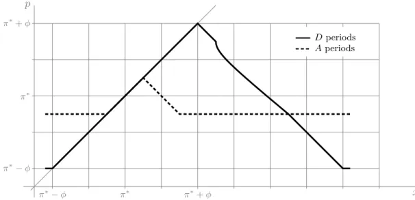
Figure 1.1: Equilibrium policy with implicit status-quo

π∗ = 2, φ= 1, δ= 0.5, rd= 0.5

x p

π∗+φ

π∗+φ π∗

π∗ π∗−φ

π∗−φ

Aperiods

D periods

effect we are ruling out cases where the ‘future looms large’ asδ approaches

unity. When this happens the requirement onC’s proposals under CS-MPE,

to bring P to indifference between accepting and rejecting when unable to propose the unconstrained maximum of her overall utility, might fail in D

periods. Intuitively, with δ large C focuses primarily on her bargaining

position captured by the VC function when determining which policy to

propose. With the VC function non-monotone, C might propose a policy

strictly inside AD, in effect disregarding her instantaneous utility. When

this happen the equilibria become cumbersome to characterize due to non-continuity of VP so that we rule those cases out by assumption.

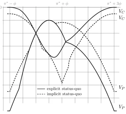
To see how the equilibrium from proposition1.1looks in graphical form, figure1.1shows a particular parametrization forπ∗= 2, φ= 1, δ= 0.5, rd=

0.5. While proving proposition 1.1we show that depending on the values of

δ and rd, the equilibrium falls into one of four (mutually exclusive) cases.

For all four of those cases the A period proposed policypA(x) has exactly

the same shape as the one given in the figure, with the constant part given

byγCA evaluated at particular values of{δ, rd}.

However, there are case dependent differences regarding the shape of the

(38)

constant and then linear increasing part for low values of x. Nevertheless, the default option x for which pD(x) reaches a maximum in general differs

depending on the values ofδ andrdand the ‘right’ part ofpD(x) (decreasing

part in figure 1.1) is not necessarily monotone or even continuous. One common feature is that it eventually decreases to γCD where it becomes a

constant function again.

Figure1.1(and proposition1.1) shows that the equilibrium shares several features with the equilibrium in the two period version of the model. It is a

CS-MPE,P is indifferent between accepting and rejecting unlessCproposes the unconstrained maximizer of her utility. Furthermore, A periods are in

effect lesser disagreement periods with degree of conflict captured by φδrd

and the committee members are failing to agree onπ∗, common bliss point in their instantaneous utility functions. Basic intuition for this result is again

the dual role of policy under the implicit status-quo bargaining, it enters

policy makers’ instantaneous utility while at the same time determining their bargaining position. On the other hand it is the Aperiods during which C

forgoes her bargaining position. By proposing pA(x) closer to π∗ relative

to the default option x, she compromises her intertemporal preferences in exchange for the current ones. Dperiods are then truly disagreement periods

and C is fully using her proposal power to steer policy towards her most

preferred one.

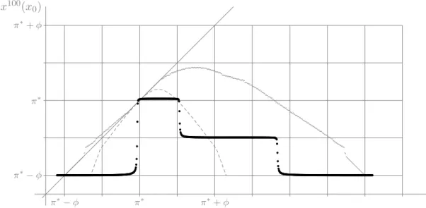
In order to discuss the long-term policy outcomes generated in

equilib-rium, we find it helpful to define a set of default options x which, when

reached, implies a constant path of default options irrespective of the type of period. Constant default options then imply policies alternating between

two (not necessarily) different values, one forAperiods and the other forD

periods. We call such a set a set ofstable default options and define it along with two notions of efficiency in the following definition.

Definition 1.4 (Stable default options and efficiency). Set S ⊆X defined by

S ={x∈X|qA(x) =qD(x) =x}

is called set of stable default options (stable set). We say bargaining displays A-efficiency whenever

(39)

We say bargaining displays D-efficiency if

pD(x) =p∗

for some p∗ ∈[π∗−φ, π∗+φ] acrossD periods.

The rationale behind the definition of stable set is that once the

bar-gaining reaches x ∈ S, resulting status-quo outcomes are constant forever for any path ofAandDperiods. If additionally we have pA(x) =pD(x) for

all x∈S we can say that the bargaining outcomes are unresponsive to the changing preferences of the committee members.

Our notion of efficiency then comes from a static Pareto efficient

mech-anism implementing an infinite sequence of policies in the current environ-ment. As we show in appendix1.A2, such a mechanism implementsπ∗ inA

periods andp∗∈[π∗−φ, π∗+φ] in Dperiods. The notion ofA-inefficiency

whenever pA(x) 6= π∗ comes from the fact that the policy makers fail to

agree on their current-period most preferred policyπ∗ due to their concerns

about their bargaining position in the future. GivenAperiod and defaultx

such that pA(x)6=π∗, if they could sign a binding contract specifying that

the next period default option will bexirrespective of today’s policy (which

they would set to π∗), both of them would be made better off. The notion

ofD-inefficiency on the other hand stresses the fact that both policy makers have a preference for policy smoothing. Finally, note that our notion of

A-efficiency looks at eachAperiod individually whileD-efficiency compares

policy decisions reached in different Dperiods.

Discussing equilibrium policy outcomes is further complicated by the fact

that those will in general depend on the default x with which bargaining

starts and on the path ofAandDperiods which is stochastic. Nevertheless, denoting byxt(x)∈X the default option aftertperiods of equilibrium play starting with default option x and some path of A and D periods, the

following proposition captures the key features.

Proposition 1.2 (Policy outcomes with implicit status-quo). CS-MPE from proposition1.1generates policy and status-quo decisions satisfying fol-lowing.

(40)

2. If x∈S thenpA(x) =pD(x)∈[π∗−φδrd, π∗+φδrd]

For initial default option x0 being continuous random variable with pdf

f(x0) defined onX, for anyt= 1,2, . . .

3. R_x

0∈XP(x

t₍_x

0)∈/S)f(x0)dx0 ≤rt_d

4. R_x

0∈XP(pA(x

t₍_x

0)) =π∗)f(x0)dx0= 0 unless rd= 0. Proof. See appendix1.A1.

Recalling the equilibrium in figure 1.1the intuition behind the result is straightforward. For any default option x ∈ S we have policies constant not only in Dperiods (part one) but also in A periods (part two). For the

third part, for any default optionxinAperiod, policy and hence status-quo

reachesS immediately and can stay out ofS only for the path ofDperiods with the probability oftconsecutiveDperiods beingrt_d. The last part then comes from the fact that the set of default options in X that can bring π∗

as a policy outcome in the future for some combination ofAand Dperiods has zero measure.

What proposition 1.2 says is that in CS-MPE from proposition1.1 un-der the bargaining protocol with implicit status-quo, bargaining outcomes eventually become stable for any distribution of initial default option (part

three). When this happens the policy outcomes display D-efficiency (part

one) on the one hand but become unresponsive to the changing preferences of the two policy makers on the other (part two) with the policy constant

henceforth. At the same time, unlessrd= 0 for any distribution of initial

de-fault option the chance that the bargaining satisfiesA-efficiency is zero both

on the path toS and once it is reached (part four). In other words, in the

CS-MPE under the implicit status-quo bargaining there is no equilibrium force that would bring the bargaining outcome eventually toA-efficiency.

Equilibrium with explicit status-quo

We now show how policy outcomes change when C’s proposals are not

re-stricted to those with policy and status-quo equal. The first result we prove is that policy in A periods is equal toπ∗ for any default option. The logic

behind the result is that since in the A periods the preferences of the two

(41)

they should not be able to reach an agreement onπ∗, as doing so needs not compromise their bargaining position embodied in status-quo. The intuition

is confirmed by the proposition.

Proposition 1.3 (pA(x) with explicit status-quo). In any S-MPE for any default option x∈X

pA(x) =π∗.

Proof. See appendix1.A1.

A key strength of proposition 1.3is that it applies to any S-MPE under the explicit status-quo bargaining protocol and shows that this bargaining

protocol allows the committee members to reach consensus in A periods.

What the proposition does not ensure is existence of such S-MPE, which is what the next proposition does.

Proposition 1.4 (S-MPE with explicit status-quo). Assume δ ≥ 1 5rd, δ ≥ 1−r_d2 and δ≤1−(1−rd)2

2 . Then there exists a unique CS-MPE in terms of associated value functions VC andVP. Equilibrium proposals satisfy

1. pA(x) =π∗ for ∀x∈X

2. VC(x)≤VC(qA(x))for ∀x∈X

3. VC(qD(x))≤VC(qD(x0))for x, x0 ∈X satisfying AD(x)⊆AD(x0) 4. C proposes γCD (γCA) for ∀x ∈ X such that γCD ∈ AD(x) (γCA ∈

AA(x))

where γCD = {π∗ −φ, z} and γCA = {π∗, z0} for some z, z0 ∈ X\(π∗ −

φ, π∗+ 3φ).

Proof. See appendix1.A1.

In words, equilibrium under explicit status-quo bargaining involves

pol-icy equal to π∗ in A periods (part one) withC using A periods to improve her bargaining position (part two). BecauseC can improve her bargaining

position inA periods, she is willing to surrender more of it in D periods in

whichP has more bargaining power (part three). Finally,C’s unconstrained proposals areγCA and γCD inA and D periods respectively, implementing

C’s instantaneous utility bliss point and status-quo that maintains her

(42)

The idea of the proof is similar to the proof of proposition 1.1. For the existence part we partially characterize the equilibrium, conjecturing

first that we are characterizing CS-MPE. This gives us theVP function and

associated acceptance sets AA and AD. We prove these are well behaved,

which allows us to prove existence of C’s continuation value function VC

as a solution toC’s dynamic optimization program (1.1). We then confirm that the proposal strategies generated by VC indeed satisfy definition 1.3

of CS-MPE. Uniqueness in terms of associated value functions then follows

from the uniqueness ofVP in any CS-MPE and resulting uniqueness of VC.

The key difficulty in the proof of proposition 1.4 and the source of the assumptions on{δ, rd}is confirming that proposal strategies associated with

VC indeed satisfy the definition of CS-MPE. What we need to ensure is that

intertemporal incentives are strong enough (first two conditions) so that C

is willing to use the status-quo dimension of her proposal space inAperiods

to bring P to indifference between accepting and rejecting as the definition of CS-MPE demands. On the other hand we need to make sure that the

intertemporal incentives are not too strong (third condition). When this

happens, inD periods P is willing to accept a wide range of policies when offered an even slightly more favourable status-quo compared to the default

option. One of those policies isC’sD period most preferred policyπ∗−φ.

With proposals involving π∗ −φ policy possibly violating requirements of CS-MPE, we need to make sure thatC foregoes only little of her bargaining

position exactly for those values of {δ, rd}, somewhat paradoxically, when

the bargaining position is most valuable.

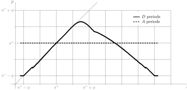
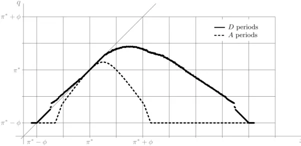
Figures 1.2 and 1.3 show equilibrium proposals from proposition 1.4 on the policy and status-quo dimension respectively for the same values

of parameters used in figure 1.1. Even though we do not have an explicit expression forVC we use computer simulation to estimateVC and associated

equilibrium proposal policies (see appendix1.A3for details of the numerical simulation). From proposition 1.4 we know that proposals on the status-quo dimension need not be unique and involve z, z