Skewness Corrected Control Charts for Random Queue Length

Skewness Corrected Control Charts for Random Queue

Length

Manik Khaparde*, Nanda Rajput **

*

Department of Statistics, P.G.T.D, R.T.M. Nagpur University, Nagpur, India.

**

Department of Statistics, M.E.S’s Abasaheb Garware College, Karve Road, Pune 411 004, India.

Abstract- Classical Shewhart kind control charts are based on normality assumption and ignore the skewness of the plotted statistic in the construction of control charts. Generally the skewness is large enough to be overlooked and in such situation the traditional chart is improper to give satisfactory performance. In this paper, we present a comparative study and present best control chart based on skewness and kurtosis for random queue length for M/M/1 queueing model evaluated on the basis of performance measure false alarm rate.

Index Terms- Control limits, false alarm rate, Haim Shore method, kurtosis correction method, (M/M/1): ( queueing system, Shewhart method, skewness correction method, skewness and kurtosis correction method

1. INTRODUCTION

Q

(i) Some measure of waiting time that a customer might be forced to bear that is the time a customer spends in the queue and the

total time a customer spends in the system (queue plus service).

(ii) The number of customers in the queue and the total number of customers in the system.

(iii) A measure of facility utilization.

As most queueing systems have stochastic elements, these measures are often random variables and their probability

distributions or their average values are desired. Depending on the type of system under study, one may be of more interest than the

other. The problem is to find out the values of appropriate measures for a given system, which quantifies the phenomenon of waiting

in queues that is the average number of customers in queue, average waiting time in queue/system and average facility utilization.

Thus average queue length and average waiting time are the main observable characteristics of any queueing system. In this paper,

control charts are proposed for the monitoring of random queue length of (M/M/1): ( queueing systems. A service system

in which customers arrive at random to avail service is known as queueing system and if a server is busy then the customer has to

wait, resulting in a queue. The customer waiting in queue is served when a server becomes available according to first come, first

serve queue discipline. The characterizing feature of a single server queue is that both the inter-arrival time and the service times are exponentially distributed with parameters λ and µ respectively. Further there is no limit to queue size. Let random variable (r.v.) N denote the number of customers in the system (either served or waiting). In this paper control charts are constructed for N by various

methods which can serve as follows:

1. To monitor the stability of the queueing system in terms of N where an out of control signal signify change in any of the

parameter that determine N say traffic intensity or in arrival or service rate of the system or rise in variance.

2. The upper control limit of N can be taken as upper patience limit of a customer in queue which can be used further in

3. In case these control limits are informed beforehand to customers, then abandonment of service by customer because of

impatience reduces. Performance of any queueing system is judged to be satisfactory if a customer has to wait for minimum

period of time within his/her patience limit in the system to get service, in concise queue length should be small.

All of the cases discussed above rely heavily on the goodness of the control chart limits [8]. Mean, standard deviation,

skewness and kurtosis are used in calculating the control limits. It is also assumed that the control charts relate to individual

observations. Through numerical analysis of the performance measure, control charts obtained by different methods are compared to

find the best performing control chart.

2. Literature Review

Control charts are one of the powerful tools of statistical process control, widely accepted and applied in industry. Basically used to

improve productivity, prevent defects and unnecessary process adjustments, also provides information in diagnosis and process

capability. Control chart effectiveness is based on control limits to detect whether a process is in control. The traditional charts are

based on the assumption that the distribution of the quality characteristic is normal or approximately normal [2]. However, in many

situations this normality assumption of process population is not valid when the process distribution is found to be skewed.

If the underlying process distribution is skewed, then methods with which false alarm rates can be controlled to the desired

level for an arbitrary skewed distribution are required. A great deal of literature developed various methods to deal with skewness of

process distribution. Chan and Cui [2] took the degree of skewness of the underlying process distribution and proposed skewness

correction (SC) method for constructing control charts for skewed distribution. Kurtosis correction method was developed to set up

control charts for the symmetric and leptokurtic distribution [8]. A skewness and kurtosis correction (SKC) method was proposed to

derive control charts with no assumption of the underlying process distribution, that takes into account the degree of skewness and

kurtosis of the process distribution and provides the control limits using three standard deviation and adding the known function of

skewness and kurtosis [9].Control charts for attributes data were developed, where the monitoring statistic may have a skewed

distribution and implemented for the study of queue length of M/M/s system [7].This paper uses control charts developed through

heuristic methods with no assumptions on the process distribution for obtaining upper control limit for characteristic i.e. number of

customers in the queueing system. Performance of control charts are judged on the basis of false alarm rate.

3. Probability distribution of the system size N

(M/M/1): (∞/FCFS) is taken for study as it models a large number of queueing problems has Poisson input, exponential service time, single server with first come, first serve queue discipline and infinite capacity. In the construction of control chart for N,

characteristics of distribution of r.v. N is needed.

Let r.v. N be the number of customers in the system (both waiting and in service) in steady state. The steady state probability

distribution of r.v. N is given by, where (1)

and is the traffic intensity or utilization rate for single server queue, λ is the mean arrival rate and µ is the mean service

rate.The r.v. N follows geometric distribution with parameter The distribution of the r.v. N depends on two parameters λ and µ only through their ratio. The model clearly suggests that, if control is possible, the parameters should be adjusted to make ρ approach 1, in order to achieve full utilization of the server.

3.1. Distributional properties of random variable N

The distributional properties of r.v. N namely mean, variance, skewness and kurtosis are displayed in the table given below.

E(N) V(N)

From the above table, it can be noted that various characteristics of N depends on traffic intensity ρ.

4. Numerical analysis of characteristics of distribution of r.v N

To study the effect of traffic intensity on the distributional properties of random variable N, a set of increasing values of ρ are selected mean, variance, skewness and kurtosis are computed and displayed in Table II. From this table, it is noted that as the values of traffic intensity (ρ) increases, the mean and variance increases rapidly. But for large values of ρ, the rate of increment in variance as compared to mean is larger, as such the expected value of N does not appear to have much relevance for large values of ρ. Although these quantities can be made arbitrarily large for sufficiently large ρ (<1), the system may therefore take long time to reach steady state equilibrium. It is observed that skewness, and kurtosis of the distribution of r.v. N decreases with increasing values of traffic

intensity.

Table II: Mean, Variance, Skewness, and Kurtosis of r.v. N

ρ E(N) V(N)

0.1 0.11111 0.123 3.47851 14.1

0.2 0.25 0.313 2.68328 9.2

0.3 0.42857 0.612 2.37346 7.633333

0.4 0.66667 1.11 2.21359 6.9

0.5 1 2 2.12132 6.5

0.6 1.5 3.75 2.06559 6.266667

0.65 1.85714 5.31 2.04657 6.188462

0.7 2.33333 7.78 2.03189 6.128571

0.75 3 12 2.02073 6.083333

0.8 4 20 2.01246 6.05

0.85 5.66667 37.8 2.00661 6.026471

0.9 9 90 2.00278 6.011111

0.91 10.1111 112 2.00222 6.008901

0.92 11.5 144 2.00174 6.006957

0.93 13.2857 190 2.00132 6.005269

0.94 15.6667 261 2.00096 6.00383

0.95 19 380 2.00066 6.002632

0.96 24 600 2.00042 6.001667

0.97 32.3333 1080 2.00023 6.000928

0.98 49 2450 2.0001 6.000408

0.99 99 9900 2.00003 6.000101

0.991 110.111 12200 2.00002 6.000082

0.992 124 15500 2.00002 6.000065

0.993 141.857 20300 2.00001 6.000049

0.995 199 39800 2.00001 6.000025

0.996 249 62300 2 6.000016

0.997 332.333 111000 2 6.000009

0.998 499 250000 2 6.000004

0.999 999 999000 2 6.000001

5. Construction of control charts for random variable N

Knowing the characteristics of the probability distribution of r.v. N control charts are constructed for N using different

methods. These charts will be referred as C-charts. As the probability function of a geometric distribution is a monotonously

decreasing function in n and since control limits for queueing system are to be computed, it would be meaningless to define lower

control limit ( LCL) for this distribution, however, obtaining upper control limit i.e. UCL would obviously make sense. Since, it will

help in monitoring improbable high values of N (the monitoring statistic) and further help in controlling abandonment due to impatience. Hence, in all control charts defined for N, only UCL, αu and ARL would be computed. The criteria used for out of control condition will be whenever a point falls outside the UCL, the system is said to be out of control. In other words, customers are running

out of patience and might abandon the system. And hence investigation and corrective action are required to be taken to find and

eliminate the causes responsible for this behaviour [6].

5.1. Control chart C1: Shewhart method

The conventional Shewhart type control charts are used to determine whether a process is in a state of statistical control to

bring out-of-control process into in-control and to monitor the process to confirm that it stays in control [5]. The limits are constructed

by assuming that the underlying distribution is normal or approximately normal. Here, control chart can be used for on-line system

surveillance and to improve the system.

Control limits for C1-chart for r.v. N when parameters are known [6]:

(2)

where E(N) and V(N) are displayed in Table

I

standard deviation units.

Control limits are used in determination of a performance measure of queueing system, hence a need for better performing

charts.

5.2. Control chart C2 : Skewness correction (SC) method

Skewness correction method corrects the Shewhart chart according to the degree of skewness of the distribution of r.v. N. It

provides asymmetric control limits using ±3 standard deviations plus the same known function of the degree of skewness estimated

from subgroups, and with no assumptions on the distribution.

The skewness correction C2 chart is based on the following control limits, when parameters are known [2]:

where denote skewness correction and is given by and E(N) , V(N) and are displayed in Table

I

, the SC chart reduces to the Shewhart chart. However, if the distribution is positively skewed, then the distance of the UCL

from the CL is larger than that of the LCL from the CL. If the distribution is negatively skewed, then the distances are reversed, but

the bandwidth of the control chart is always six.

5.3. Control chart C3: Haim Shore method

Sometimes the skewness is too large to be ignored and may be crucial to the proper functioning. Ignoring skewness affects

the performance of the control chart and results in raised Type I risk. These findings have instigated in the development of various

control charts that takes into consideration the non-normality of the monitoring statistic. Control charts for attributes data were

developed, where the monitoring statistic may have a skewed distribution and implemented it for the study of queue length of M/M/s

system[7]. Unlike the traditional chart which uses only standard normal quantiles, the control chart for attributes may use logistic

quantiles. Since this may help for monitoring statistic with exceptionally high skewness and high kurtosis.

The control limits for N, obtained by Haim Shore method which involves the first three moments of the r.v. N are:

(4)

(5)

(6)

where E(N),V(N) and are displayed in Table

I

II

the skewness of the distribution of N decreases as ρ increases. Also, the minimum value of skewness is nearly 2 which are observed for high values of ρ. Therefore control limits given by expressions (4), (5) and (6) are used, as the distribution of N is highly skewed and for high values of skewness the probability limits, based on normal quantiles, may not be appropriate due to the long tails

associated with highly skewed distributions or distributions that do not converge to the normal. Hence, control limits based on the

logistic quantile are used which are proved to be more efficient, as it has longer tails relative to normal variable.

5.4. Control chart C4 : Kurtosis correction (KC) method

Tadikamalla and Popescu [8] developed a KC method to construct control chart when the process distribution is symmetrical,

but is leptokurtic, it has the advantage of providing better control limits and are easier to use and make no assumption on the

functional form of underlying distribution. This method shifts the control limits to both sides by the same amount which is function of kurtosis, which is estimated by sample kurtosis. It is observed that the use of the α-quantile of the normal distribution is not appropriate, if the process distribution is skewed.

The control limits based on KC method for C4 control chart if the process distribution and parameters are known for r.v. N

(7)

where E(N),V(N) and are displayed in Table

I

Shewhart chart.

5.5. Control chart C5 : Skewness and kurtosis correction (SKC) method

Wang (2009)[9] developed a SKC method to construct control chart with no assumptions on the process distribution, both the

degree of skewness and kurtosis of the process distribution is taken into account. It provides the control limits using 3 standard

deviation with addition of the known function of skewness and kurtosis. If kurtosis of the process distribution is zero then SKC

method reduces to SC method and to Shewhart if both skewness and kurtosis of the distribution are found to be zero.

The control limits based on SKC method if the process distribution and parameters are known for r.v. N ,

(8)

where E(N),V(N), and are as displayed in Table

I

6. Performance measures

In this section performance measures of control chart are studied.

6.1. False alarm rate for control chart

Let αu denote the probability of type I error generated in the upper tail of the control chart. The Type-I error rate is defined as the probability of signalling an out of control even though the process is actually in-control. It is defined as, αu= =ρUCL where UCL is as obtained for control charts based on different methods. This implies that the probability of exceeding some limit on

the number of customers in the system is a geometrically decreasing function of that number and decays very rapidly.

6.2. Average run length

Let ARLCi, i=1,…,5 denote the average run length of control chart Ci. ARL is the average number of points that must be

plotted before a point indicates an out of control condition. If the system observations are uncorrelated, then for any control chart; the

average run length is given by [6],

, i=1,…,5 where αu is the false alarm rate . (9)

7. Performance comparison of different control charts

The control limits of control chart based on different methods depend on traffic intensity ρ. To study the effect of ρ on control limits and performance measures, same set of increasing values of ρ are selected and CL, UCL,FAR and ARL were computed and comparisons were carried out.

i. When ρ=0.1 and 0.2 , 3.48 and 2.68 and and 9.2

respectively, it is observed that,

< .

Consequently,

> .

As UCL of control chart based on KC method is found to be highest of all methods, so corresponding FAR is lowest and

consequently ARL is highest. Whereas, UCL obtained by Shewhart method is lowest, so FAR is found to be highest and resultantly

ARL is lowest of all the methods. The argument is as the underlying distribution is highly skewed and leptokurtic, the FAR is large as

skewness is high and also because of the discrepancy between the variability pattern of the asymmetric distribution and the normality

assumed in constructing the control chart.

ii. For , 2.37 to 2 and to 6,it is observed that,

< .

Consequently,

> .

FAR obtained from control chart based on Haim Shore method is lowest consequently the ARL is highest of all methods and lowest

for Shewhart method. Hence control chart based on Haim Shore method is best of all, second best is control chart based on KC

method and third best under this situation is control chart based on SKC method.

iii. From Table II, it is observed that for skewness around 2, traffic intensity is nearer to 1.From figure 2 it is observed that as skewness decreases FAR decreases whereas ARL increases(observe figure 4) .On the other hand from figure 1 as traffic intensity(ρ) increases FAR decreases whereas ARL increases(observe figure 3). On the basis of FAR, control charts C3, C4 and C5 show

comparable performance.

Table III: Comparison of False Alarm Rate of control charts based on various methods

0.1 3.47851 0.06836 0.02282 0.009803 0.00909 0.018728

0.2 2.68328 0.04498 0.01203 0.006205 0.00579 0.00968

0.3 2.37346 0.03536 0.0087 0.004562 0.00458 0.006945

0.4 2.21359 0.02994 0.0071 0.003604 0.00392 0.005636

0.5 2.12132 0.02641 0.00614 0.002972 0.00348 0.004862

0.6 2.06559 0.0239 0.0055 0.002523 0.00317 0.004345

0.65 2.04657 0.02289 0.00525 0.002344 0.00304 0.004145

0.7 2.03189 0.02201 0.00503 0.002187 0.00293 0.003973

0.75 2.02073 0.02122 0.00484 0.002049 0.00283 0.003822

0.8 2.01246 0.02052 0.00467 0.001926 0.00274 0.00369

0.85 2.00661 0.01989 0.00453 0.001816 0.00265 0.003572

0.9 2.00278 0.01932 0.00439 0.001718 0.00258 0.003466

0.91 2.00222 0.01921 0.00437 0.001699 0.00256 0.003447

0.93 2.00132 0.019 0.00432 0.001663 0.00254 0.003408

0.94 2.00096 0.01889 0.0043 0.001646 0.00252 0.00339

0.95 2.00066 0.01879 0.00427 0.001628 0.00251 0.003371

0.96 2.00042 0.0187 0.00425 0.001612 0.0025 0.003353

0.97 2.00023 0.0186 0.00423 0.001595 0.00248 0.003336

0.98 2.0001 0.0185 0.00421 0.001579 0.00247 0.003319

0.99 2.00003 0.01841 0.00418 0.001563 0.00246 0.003302

0.991 2.00002 0.0184 0.00418 0.001561 0.00246 0.0033

0.992 2.00002 0.01839 0.00418 0.00156 0.00246 0.003298

0.993 2.00001 0.01838 0.00418 0.001558 0.00245 0.003297

0.994 2.00001 0.01837 0.00418 0.001557 0.00245 0.003295

0.995 2.00001 0.01836 0.00417 0.001555 0.00245 0.003293

0.996 2 0.01835 0.00417 0.001554 0.00245 0.003292

0.997 2 0.01834 0.00417 0.001552 0.00245 0.00329

0.998 2 0.01833 0.00417 0.00155 0.00245 0.003289

0.999 2 0.01833 0.00417 0.001549 0.00245 0.003287

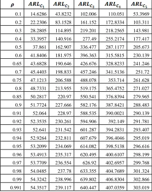
Table IV: Comparison of Average Run Length (ARL) of control charts based on various methods

0.1 14.6286 43.8232 102.006 110.051 53.3969

0.2 22.2306 83.1528 161.152 172.8334 103.311

0.3 28.2805 114.895 219.201 218.2565 143.981

0.4 33.3957 140.916 277.49 255.2174 177.417

0.5 37.861 162.907 336.477 287.1177 205.673

0.6 41.8406 181.975 396.363 315.5815 230.139

0.65 43.6828 190.646 426.676 328.8233 241.246

0.7 45.4403 198.833 457.246 341.5136 251.72

0.75 47.1213 206.588 488.078 353.714 261.628

0.8 48.7331 213.955 519.175 365.4752 271.027

0.85 50.2817 220.97 550.541 376.8394 279.965

0.9 51.7724 227.666 582.176 387.8421 288.483

0.91 52.064 228.97 588.535 390.0021 290.139

0.92 52.3535 230.261 594.906 392.149 291.781

0.93 52.641 231.542 601.287 394.2831 293.407

0.94 52.9264 232.811 607.679 396.4046 295.019

0.95 53.2099 234.069 614.082 398.5138 296.616

0.96 53.4913 235.317 620.495 400.6107 298.199

0.97 53.7709 236.554 626.92 402.6957 299.768

0.98 54.0485 237.78 633.355 404.7689 301.324

0.99 54.3242 238.996 639.802 406.8304 302.866

0.992 54.3792 239.238 641.092 407.2413 303.172

0.993 54.4066 239.359 641.738 407.4466 303.326

0.994 54.434 239.48 642.383 407.6518 303.479

0.995 54.4614 239.601 643.029 407.8568 303.632

0.996 54.4888 239.721 643.675 408.0618 303.784

0.997 54.5162 239.842 644.321 408.2666 303.937

0.998 54.5435 239.962 644.967 408.4713 304.09

0.999 54.5708 240.082 645.613 408.676 304.242

Figure 1 Figure 2

8. Conclusion

The paper proposes performance wise for =0.1 and 0.2 use of control chart C4 based on KC method, since it outperforms rest methods. Further for ρ>0.3 the use of control chart C3 based on Haim Shore method for obtaining UCL for random queue length (N). Since C3 out performs charts based on all other methods as it considers in its construction of control limits skewness of underlying distribution of r.v. N. This control chart can be suggested for intimating system management for taking precautionary measure. Hence control chart C3 is recommended for skewed population and KC method C4 as next best of all charts. For a process in control, the ARL is preferred to be large because an observation plotting outside the control limits represents a false alarm. R software was used in computation.

REFERENCES

[1] D.S. Bai, and I.S. Choi,” and R control charts for skewed populations,” Journal of Quality technology,1995, Vol. 27, No. 2,pp. 120-131. [2] L.K .Chan, and H.J. Cui,” Skewness correction and R charts for skewed distributions,” Naval Research Logistics, 2003, 50, No. 6,pp. 555-573.

[3] Y.S. Chang, and D. S. Bai,” Control charts for positively-skewed populations with weighted standard deviations,” Quality and Reliability Engineering International, 2001, 17:397-406. (DOI:10.1002/ qre.427).

[4] K .Derya, and H.Canan, ” Control charts for skewed distributions: Weibull, gamma, and lognormal,” Metodoloski zvezki, 2012, Vol. 9, No. 2: pp. 95-106. [5] M.B.C.Khoo, A.M. Atta, ,”An EWMA control chart for monitoring the mean of skewed populations using weighted variance,” Proceedings of the 2008 IEEE

IEEM.

[6] D.C.Montgomery, Statistical Quality Control: A Modern Introduction. Sixth edition. Wiley- India Edition,2010, India [7] H.Shore,” General control charts for attributes,” IIE Transactions,2000, 32: 1149-1160.

[8] P.R.Tadikamalla, D.G. Popescu,,” Kurtosis correction method for and R control charts for long-tailed symmetrical distributions,” [Online]. Wiley Inter Science. Available: www.interscience.wiley.com. Wiley Periodicals, Inc. Naval Research Logistics,17 January 2007, 54:371-383

.

[9] S.B.Wang,” Skewness and kurtosis correction for and R control charts,” Institute of Statistics, National University of Kaohsiung,2009, Kaohsiung, Taiwan 811 R.O.C..

AUTHORS

First Author –MANIK KHAPARDE, Ph.D., Department of Statistics, P.G.T.D, R.T.M. Nagpur University, Nagpur, India

mvkkhaparde@yahoo.co.in

Second Author – NANDA RAJPUT, M.Sc., M.Phil.,M.E.S’s Abasaheb Garware College, Karve Road, Pune 411 004, India, and

nandarajput@yahoo.com