Combined Real and Reactive Power Economic Dispatch using Multi-Objective Reinforced Learning with Optimized Losses

Combined Real and Reactive Power Economic Dispatch

using Multi-Objective Reinforced Learning with

Optimized Losses

Moses Peter Musau, Nicodemus Odero Abungu, Cyrus Wabuge Wekesa

Department of Electrical and Information Engineering, School of Engineering, The University of Nairobi, Nairobi, Kenya

Abstract- Most of the economic dispatch (ED) works so far deal with real power dispatch only. With the integration of renewable energy into the grid, reactive power dispatch cannot be ignored any longer due to its importance in providing security and reliability in power system planning, operation and control. This paper deals with the formulation of combined real and reactive economic dispatch (CRRED) subject to equality, inequality and stochastic constraints. An effective algorithm that uses a hybrid of distributed slack bus (DSB) formulated using combined participation factors (PF) and multi objective reinforcement learning (MORL) is proposed in this paper. The IEEE 14 Bus was used to validate the effectiveness of the proposed CRRED formulation and Hybrid method .The numerical results obtained show that combining real and reactive power results in a 0.95% decrease in the overall generation cost as compared to a case in which only real power is considered. Further, when the losses are distributed in the entire network using the DSB, then the overall generation cost is reduced by 29.6% due to the reduced losses in DSB model.

Index Terms- Combined Real and Reactive Economic Dispatch (CRRED), Distributed Slack Bus (DSB),Participation Factors (PF), Reinforcement Learning (RL)

I. INTRODUCTION

eactive power production is highly dependent on the real power output. However, reactive power production by a generator reduces its capability to produce active power. Hence the production of reactive power by generator will result in reduction of its active power production. In addition Renewable power systems generate and absorb reactive power at the same time,leading to a stochastic reactive power scenario. Thus the place of reactive power in the modern power system cannot be ignored any longer. The objectives of reactive power (VAR) optimization, which include Reactive Power ED (RPED), are to improve the voltage profile, to minimize system active power losses, and to determine optimal VAR compensation placement under various operating conditions. To achieve these objectives, power system operators utilize control options such as adjusting generator excitation, transformer tap changing, shunt capacitors, and SVC. There has been a growing interest in VAR optimization problems over the last decade. Solving Optimal RPED (ORPED) is gaining more importance due to their effectiveness in handling the inequality constraints and discrete values using hybrid methods as compared to the deterministic and heuristic methods. Thus better method are needed to handle the more complex problems where stochastic reactive power from wind and solar generators are involved.

II. REVIEWOFREACTIVEPOWERECONOMICDISPATCH(RPED)

Various aspects of reactive power have been considered in past researches. Deterministic methods have been used in past researches to handle problems related with reactive power optimal flow .These include Unified Method (UM) by Lee, K.Y, Park Y.M, and Ortiz, J. L, 1985 [1] ,Linear Programming (LP) and Quadratic Programming (QP) by Serrano, B. R. Vargas, 2001 [2],Mean-Variance Mapping Optimization (MVMO) by Worawat Nakawiro et al, 2011 [3],Superiority of Feasible solutions (SF), Self-adaptive Penalty (SP), εε-constraint (EC), Stochastic Ranking (SR), and the Ensemble of Constraint Handling Techniques (ECHT) by R. Mallipeddi et al,2012 [4] and Second Stochastic Chance-Constrained Model (SSCCM) by Lopez, J.C. et al, 2012 [5].Heuristic methods such as Adaptive Genetic Algorithm (AGA) has also been considered by Q.H. Wu, Y.J. Cao, J.Y. Wen, 1998 [6].In all these works, the Cost function for the reactive power economic dispatch not formulated and further only Static reactive power has been considered .Thus, there is need to formulate the reactive power cost function, determine the cost coefficients and finally come up with a method in which the real and reactive costs can be combined. It can also be noted that only pure methods have been employed in this problem. These methods are strong and weak at the same time, thus there is need to use a hybrid methods which exalts the strengths and suppresses the weaknesses.

In previous studies different techniques have been suggested to determine the reactive power pricing [15-23]. For example, Niknam et al., 2004[21], utilized various search techniques such as genetic algorithm (GA) and ant colony algorithms (ACO) for pricing and Chung et al. 2004[23] proposed a coupled market framework for energy and reactive power. Further, Bialek and Kattuman,2004 [22] developed an integrated method to calculate both real and reactive power spot price and to decompose them into the prices of selected ancillary services.

III. PROBLEMFORMULATION

In order to obtain a more accurate cost function, the reactive power cost is to be included in the active power cost function. The total cost is given by combining the active and reactive power cost by a weighting function,giving the active power more weight than the reactive power.

Real Power Dynamic Economic Dispatch

For real power,dynamic economic dispatch (DED) considers change-related costs. The DED takes the ramp rate limits, valve points and prohibited operating zone of the generating units into consideration. The general form of DED was formulated by Yusuf Somez, 2013[7] as is given by

where are the cost coefficients of the unit, is the lower generation bound for the unit

and is the error associated with the equation. The problem is solved subject to the following constraints:

Reactive Power Economic Dispatch

According to Hasanpour, S., et al 2009[15] the fuel cost function for the reactive power output can be expressed as

Where and are the reactive power cost coefficients calculated using a curve fitting method, is the reactive

Power balance constraints

Continuous control variable (Generator Bus Voltage)

Discrete control variable (Transformer Tap Settings)

Where is the tap setting of transformer at branch k

State variables

Reactive power balance

In these constraints, is the reactive power generated by the capacitor bank, is the reactive power generated at bus

i, is the apparent power flow through the ith branch, is the total number of buses, the number of tap setting

transformer branches, is the number of capacitor banks and is the number of generator buses, Reactive power generated

by generator i, Reactive power generated and absorbed by VAR compensation device j such as capacitors,SVC,Wind Based

Doubly Fed Induction Generators s(DFIGs), and PV generators, Reactive power load at load bus k and Power system

reactive power power loss and absorption .Further , is the voltage magnitude at bus i , is the voltage magnitude at bus

j, is the real and reactive powers injected at bus i, is the mutual conductance and suspectance between bus i and j

Combined Real and Reactive Economic Dispatch (CRRED)

In order to obtain a more accurate optimal cost, the reactive power cost is to be included in the active power cost function. The total cost is given by combining the active and reactive power cost, giving the active power more weight than the reactive power.The CRRED objective function for dynamic reactive power is formulated as

Where W is the weight attached to the real power.

IV. MULTIOBJECTIVEREINFORCEDLEARNING(MORL)WITHDISTRIBUTEDSLACKBUS (DSB)[MORL-DSB] In the past researches, heuristic and deterministic methods haven been widely used in the real power economic dispatch[1-6,15-23] due to their ability to solve such optimization problems with speed and accuracy. Musau et al,2015 [ 24] did a detailed review of the methods that have been used so far in solving the Multi Objective Dynamic Economic Dispatch (MODED). A more recent trend for solving MODED is the two-method and three-method hybrids formulation in which all the weaknesses of the base methods (that is, deterministic and heuristic methods) are suppressed and the strengths exalted. This leads to increased accuracy and speed in handling higher order cost functions with more objectives. However, hybrid methods have not been applied to CRRRED problems. This paper utilizes a hybrid of MORL and DSB for the first time.

a) Multi Objective Reinforced Learning[MORL]

The RL used in this case has been suggested by, E. A. Jasmin et al, 2011[13].The solution consists of two phases: learning phase

and retrieval phase.To carry out the learning task, one issue is regarding how to select an action from the action space. The two

b)DSB with MORL (DSB-MORL)

Tong and K.Miu [8-11] formulated a real power DSB using the Newton Raphson Method. In this case real power participation factors (PF) were utilized to model the losses. Musau et al,2012[12] developed reactive power DSB then applied the results in [8-11] to come up with combined DSB which can handle both real and reactive power. In this paper, this combined DSB has been used to optimize the real and reactive losses, which is, compared to the Single Slack Bus (SSB) model. DSB results in reduced real and reactive power losses .MORL is then utilized to handle the CRRED in which the losses have been optimized by the DSB.

V. RESULTSANDANALYSIS

Simulations were carried out on an Intel Core i3, 2.10 GHz, 4-GB RAM processor. The coding is written in MATLAB 2013a version. A hybrid of RL-DSB algorithm was used for solving the CRRED problem. The IEEE-14 bus system used to validate the method consists of 14 buses, 5 generators and 20 lines.The results consists of four parts,a load flow for the DSB and SSB,MORL, MORL-DSB and a comparison with other methods in the existing literature.

a) SSB and DSB Load flows

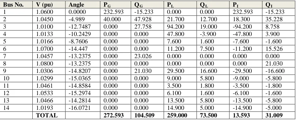
A load flow for the IEEE 14 Bus system was performed to illustrate the need for DSB,and the corresponding participation factors in CRRED problem. From tables 1.0-4.0,it is evident that DSB leads to reduced combined losses as compared to the SSB.The integration of the reactive power participation factor(RPPF) reduces the real losses to a great extent.

Table 1.0: Output Data with Single Slack Bus (SSB)

Bus No. V (pu) Angle PG QG PL QL PI QI

1 1.0600 0.0000 232.593 -15.233 0.000 0.000 232.593 -15.233

2 1.0450 -4.989 40.000 47.928 21.700 12.700 18.300 35.228

3 1.0100 -12.7487 0.000 27.758 94.200 19.000 -94.200 8.758

4 1.0133 -10.2429 0.000 0.000 47.800 -3.900 -47.800 3.900

5 1.0166 -8.7606 0.000 0.000 7.600 1.600 -7.600 -1.600

6 1.0700 -14.447 0.000 0.000 11.200 7.500 -11.200 15.526

7 1.0457 -13.2375 0.000 23.026 0.000 0.000 0.000 0.000

8 1.0800 -13.2375 0.000 0.000 0.000 0.000 0.000 21.030

9 1.0306 -14.8207 0.000 21.030 29.500 16.600 -29.500 -16.600

10 1.0299 -15.0365 0.000 0.000 9.000 5.800 -9.000 -5.800

11 1.0461 -14.8584 0.000 0.000 3.500 1.800 -3.500 -1.800

12 1.0533 -15.2974 0.000 0.000 6.100 1.600 -6.100 -1.600

13 1.0466 -14.2814 0.000 0.000 13.500 5.800 -13.500 -5.800

14 1.0193 -16.0721 0.000 0.000 14.900 5.000 -14.900 -5.000

TOTAL 272.593 104.509 259.000 73.500 13.593 31.009 Table 2. 0 :Line Flows and Losses with Single Slack Bus(SSB)

From-To P(MW) Q(Mvar)

From-To P(MW) Q(Mvar) Loss (MW) Loss(Mvars)

1-2 157.080 -17.484 2-1 -152.772 30.369 4.309 13.155

1-5 75.513 7.981 5-1 72.740 3.464 2.773 11.455

2-3 73.396 5.936 3-2 71.063 3.894 2.333 9.830

2-4 55.943 2.935 4-2 54.273 2.132 1.670 5.067

2-5 41.733 4.738 5-2 40.813 -1.929 0.920 2.890

3-4 -23.137 7.752 4-3 23.528 -6.753 0.391 0.998

4-5 -59.585 11.574 5-4 60.064 -10.063 0.479 1.511

4-7 27.066 -15.396 7-4 -27.066 17.372 0.000 1.932

4-9 15.464 -2.640 9-4 15.464 3.932 0.000 1.292

5-6 45.889 -20.843 6-5 -45.889 26.617 0.000 5.774

6-11 8.287 8.898 11-6 -8.165 -8.641 0.123 0.257

6-12 8.064 3.176 12-6 -7.9485 -3.008 0.081 0.168

6-13 18.337 9.981 13-6 -18.085 -9.485 0.252 0.496

7-8 0.000 -20.362 8-7 0.000 21.030 0.000 0.668

7-9 27.066 14.798 9-7 -27.066 -13.840 0.000 0.957

9-14 8.637 0.321 14-9 -8.547 -0.131 0.089 0.190

10-11 -4.613 -6.720 11-10 4.665 6.841 0.051 0.120

12-13 1.884 1.408 13-12 -1.873 -1.398 0.011 0.010

13-14 6.458 5.083 14-13 -6.353 -4.869 0.105 0.215

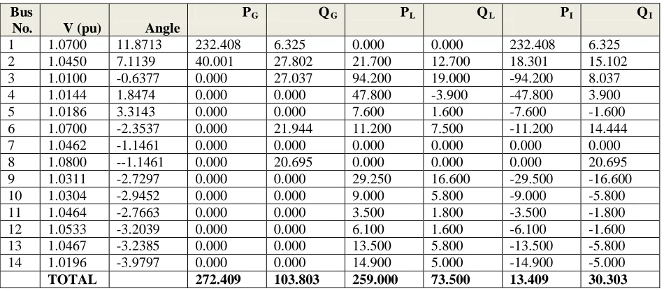
TOTAL LOSS 13.593 56.910 Table 3. 0: Output Data with Distributed Slack Bus (DSB) using Real Power PF Bus

No. V (pu) Angle

PG QG PL QL PI QI

1 1.0700 11.8713 232.408 6.325 0.000 0.000 232.408 6.325

2 1.0450 7.1139 40.001 27.802 21.700 12.700 18.301 15.102

3 1.0100 -0.6377 0.000 27.037 94.200 19.000 -94.200 8.037

4 1.0144 1.8474 0.000 0.000 47.800 -3.900 -47.800 3.900

5 1.0186 3.3143 0.000 0.000 7.600 1.600 -7.600 -1.600

6 1.0700 -2.3537 0.000 21.944 11.200 7.500 -11.200 14.444

7 1.0462 -1.1461 0.000 0.000 0.000 0.000 0.000 0.000

8 1.0800 --1.1461 0.000 20.695 0.000 0.000 0.000 20.695

9 1.0311 -2.7297 0.000 0.000 29.250 16.600 -29.500 -16.600

10 1.0304 -2.9452 0.000 0.000 9.000 5.800 -9.000 -5.800

11 1.0464 -2.7663 0.000 0.000 3.500 1.800 -3.500 -1.800

12 1.0533 -3.2039 0.000 0.000 6.100 1.600 -6.100 -1.600

13 1.0467 -3.2385 0.000 0.000 13.500 5.800 -13.500 -5.800

14 1.0196 -3.9797 0.000 0.000 14.900 5.000 -14.900 -5.000

TOTAL 272.409 103.803 259.000 73.500 13.409 30.303

Table 4.0: Line Flows and Losses with Distributed Slack Bus(DSB) using Real Power PF

From-To P(MW) P(MW)

From-To P(MW) P(MW) Loss (MW) Loss(Mvars)

1~2 156.840 0.349 2~1 -152.677 12.364 4.164 12.713

2~3 75.567 11.815 3~2 -72.807 -0.419 2.761 11.397

2~4 73.320 5.944 4~2 -70.991 3.866 2.328 9.810

1~5 55.924 2.243 5~1 -54.257 2.815 1.667 5.058

2~5 41.735 3.572 5~2 -40.820 -0.778 0.915 2.794

3~4 -23.209 7.058 4~3 23.595 -6.071 0.387 0.987

4~5 -59.725 9.739 5~4 60.200 -8.241 0.475 1.499

5~6 27.100 -15.087 6~5 -27.100 16.999 0.000 1.912

4~7 15.487 -2.515 7~4 -15.487 3.804 0.000 1.289

7~8 45.827 -20.042 8~7 -45.827 25.706 0.000 5.664

4~9 8.253 8.793 9~4 -8.132 -8.541 0.121 0.253

7~9 8.057 3.163 9~7 -7.976 -2.996 0.080 0.167

9~10 18.317 9.927 10~9 -18.066 -9.433 0.251 0.494

6~11 0.000 -20.049 11~6 0.000 20.695 0.000 0.647

6~12 27.100 14.825 12~6 -27.100 -13.866 0.000 0.959

6~13 4.424 -0.807 13~6 -4.418 0.823 0.006 0.016

9~14 8.662 0.384 14~9 -8.572 -0.192 0.090 0.191

10~11 -4.582 -6.623 11~10 4.632 6.741 0.050 0.117

12~13 1.876 1.396 13~12 -1.865 -1.386 0.011 0.010

13~14 6.432 5.019 14~13 -6.328 -4.808 0.104 0.211

Table 5.0:Line Flows and Losses with Distributed Slack Bus using Reactive Power PF

Bus

No. V (pu) Angle

PG QG PL QL PI QI 1 1.0500 12.0665 223.861 -35.774 0.000 0.000 223.861 -35.774

2 1.0450 7.0834 46.150 57.193 21.700 12.700 24.450 44.493

3 1.0200 -0.6686 2.287 37.215 94.200 19.000 -91.913 18.215

4 1.0142 1.8161 -1.790 -5.224 47.800 -3.900 -49.590 -1.324

5 1.0172 3.3072 2.114 -0.211 7.600 1.600 -5.486 -1.811

6 1.0800 -2.3425 7.030 40.454 11.200 7.500 -4.170 32.954

7 1.0503 -1.1766 -0.000 -5.963 0.000 0.000 -0.000 -5.963

8 1.1000 -1.1738 0.032 31.006 0.000 0.000 0.032 31.006

9 1.0337 -2.7573 -0.000 0.000 29.500 16.600 -29.500 -16.600

10 1.0326 -2.9662 -0.000 0.000 9.000 5.800 -9.000 -5.800

11 1.0475 -2.7727 -2.080 -4.273 3.500 1.800 -5.580 -6.073

12 1.0535 -3.1932 -1.657 -3.322 6.100 1.600 -7.757 -4.922

13 1.0471 -3.2329 -3.344 -6.339 13.500 5.800 -16.844 -12.139

14 1.0213 -3.9896 -0.000 0.000 14.900 5.000 -14.900 -5.000

TOTAL 272.603 104.762 259.000 73.500 13.603 31.262

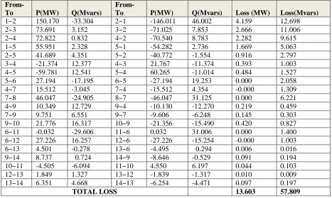
Table 6.0 :Line Flows and Losses with Distributed Slack Bus(DSB) for Combined PF

From-To P(MW) Q(Mvars)

From-To P(MW) Q(Mvars) Loss (MW) Loss(Mvars)

1~2 150.170 -33.304 2~1 -146.011 46.002 4.159 12.698

2~3 73.691 3.152 3~2 -71.025 7.853 2.666 11.006

2~4 72.822 0.832 4~2 -70.540 8.783 2.282 9.615

1~5 55.951 2.328 5~1 -54.282 2.736 1.669 5.063

2~5 41.689 4.351 5~2 -40.772 -1.554 0.916 2.797

3~4 -21.374 12.377 4~3 21.767 -11.374 0.393 1.003

4~5 -59.781 12.541 5~4 60.265 -11.014 0.484 1.527

5~6 27.194 -17.195 6~5 -27.194 19.253 0.000 2.058

4~7 15.512 -3.045 7~4 -15.512 4.354 -0.000 1.309

7~8 46.047 -24.905 8~7 -46.047 31.125 0.000 6.221

4~9 10.349 12.729 9~4 -10.130 -12.270 0.219 0.459

7~9 9.751 6.551 9~7 -9.606 -6.248 0.145 0.303

9~10 21.776 16.317 10~9 -21.356 -15.490 0.420 0.827

6~11 -0.032 -29.606 11~6 0.032 31.006 0.000 1.400

6~12 27.226 16.257 12~6 -27.226 -15.254 -0.000 1.003

6~13 4.501 -0.278 13~6 -4.495 0.294 0.006 0.016

9~14 8.737 0.724 14~9 -8.646 -0.529 0.091 0.194

10~11 -4.505 -6.094 11~10 4.550 6.197 0.044 0.103

12~13 1.849 1.327 13~12 -1.839 -1.317 0.010 0.009

13~14 6.351 4.668 14~13 -6.254 -4.471 0.097 0.197

TOTAL LOSS 13.603 57.809

From tables 4.0-6.0,it can be easily observed that ,the combined participation factors(CPF) leads to reduced losses as compared to the real power participation factors (RPF) hence the increased importance of reactive power in power loss reduction.

b) Multi Objective Reinforced Learning [MORL]

The RL parameters that were used in the algorithm are given in table 7.0: Table 7.0:MORL Parameters

0.5

0.1

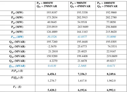
www.ijsrp.org Power scheduling was done considering the three sets of real power and reactive power demands shown in table 8.0. The optimal generation of the five generating units and the optimal cost are also tabulated as shown in Table 8.0.CRRED problem formulation and solution led to reduced fuel cost as compared to the pure real power.

Table 8.0: Real and Reactive Power Scheduling for a 14-Bus System

PD = 800MW

QD = 370MVAR

PD = 900MW

QD = 470MVAR

PD = 1000MW

QD = 570MVAR

Pg1 (MW) 193.8187 193.3338 192.9860

Pg2 (MW) 173.2834 202.5915 202.2780

Pg3 (MW) 40.9645 54.9518 77.0050

Pg4 (MW) 235.0919 243.9489 256.8600

Pg5 (MW) 126.4889 164.1163 215.8620

Ploss (MW) 30.3526 41.0577 55.0090

Qg1 (MVAR) 195.7260 195.4648 195.0305

Qg2 (MVAR) -2.5670 25.6773 74.5531

Qg3 (MVAR) 21.2810 25.4025 22.9167

Qg4 (MVAR) 150.9200 199.4408 219.0609

Qg5 (MVAR) 4.2270 21.6678 49.8217

Qloss (MVAR) 0.4130 2.3468 8.6171

F(Pgi) ($)

6,456.1 7,336.3 8,249.6

F(Qgi) ($)

1,276.7 1,617.8 1,962.0

FT ($)

5,420.2 6,192.6 6,992.1

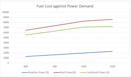
Figure 2.0: Fuel cost against Power Demand

From Figure 2.0, it is clear that the real power cost was higher than the reactive power cost. However, the combined real and reactive power cost was lower than the real power cost. This implies that the cost of generation reduces when combined real and reactive power cost is computed as compared to just considering real power generation that most economic dispatch problems involves. In Figure 2.0 , a real power demand of 800MW corresponds to reactive power demand of 370MVAR, 900MW corresponds to 470MVAR, and 1000MW corresponds to 570MVAR (x axis).

Figure 3.0: Power Losses against Power Demand

From Figure 3.0, the power losses increased with higher levels of power demanded. It is also clear that the real power losses were higher than the reactive power losses.The combined losses are a vector sum of the Real and reactive losses hence they are higher than both the two components considered separately.

0 20 40 60 80 100 120 140

800 850 900 950 1000 1050 1100

Losses againist Power Demand

c) MORL with DSB

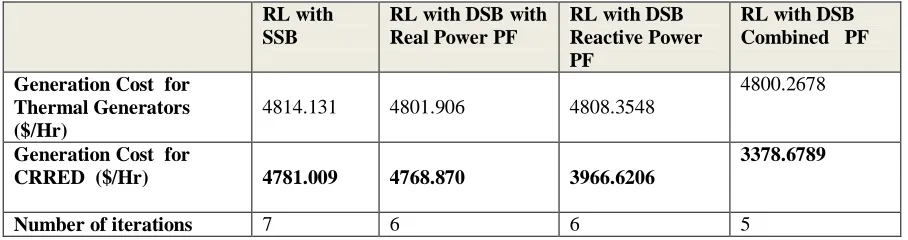
As shown in table 9.0, use of MORL with Combined PF DSB led to lower system losses as compared to the real power DSB. This is because the inclusion of reactive power in DSB leads to improve voltage profile which translates to better reactive power management. The SSB –RL has the highest system losses. The generation cost are as tabulated in Table 10.0 for CRRED problem. From this table it is clear that which the generation cost are lowest in the DSB-MORL with combined PF compared to MORL with real power DSB and SSB. Further the inclusion of reactive power in ED formulation led to reduced cost as compared to a scenario in which only real power of the thermal units is considered. The algorithm with combined PF DSB provided a feasible solution with fewer iterations as compared to the other two scenarios.

Table 9.0: Comparison of Generated Power RL with

SSB(MW)

RL with DSB using Real PF

(MW)

RL with DSB using

Reactive PF(MW)

RL with DSB With Combined

PF(MW)

Generation:

Plant 1 232.593 232.408 223.861 231.206

Plant 2 40.000 40.001 46.150 40.0000

Total System Losses 13.593 13.409 13.603 13.301

Table 10.0: Comparison of Generation Costs in MORL-DSB RL with

SSB

RL with DSB with Real Power PF

RL with DSB Reactive Power PF

RL with DSB Combined PF Generation Cost for

Thermal Generators ($/Hr)

4814.131 4801.906 4808.3548

4800.2678

Generation Cost for

CRRED ($/Hr) 4781.009 4768.870 3966.6206

3378.6789

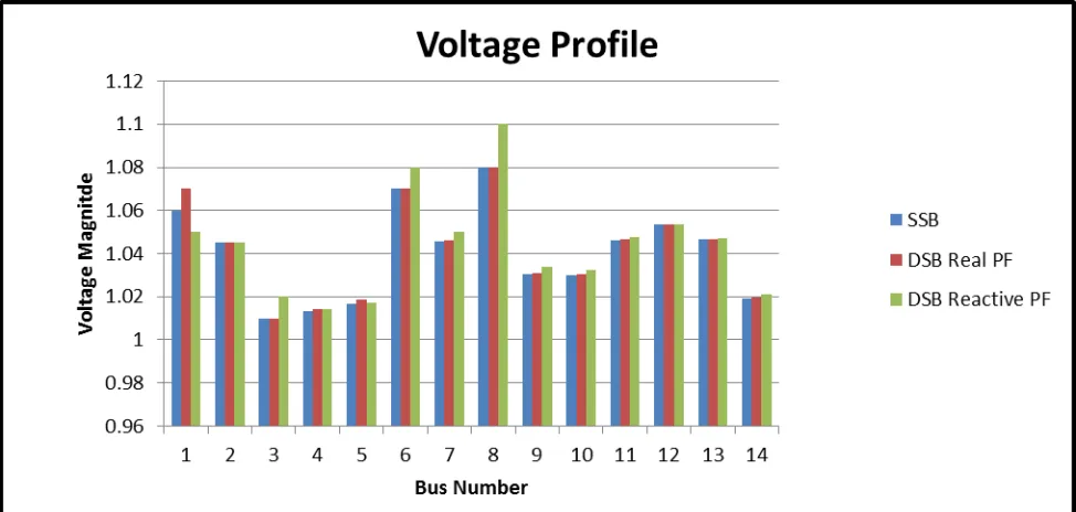
Figure 4.0 :Voltage Profile Comparison

Figure 6.0: Comparison of Real Power Generation

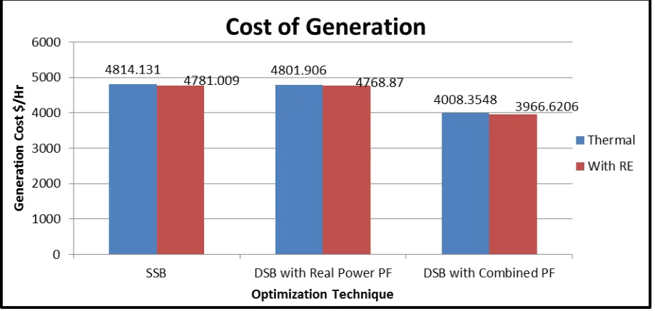
Figure 7.0: Comparison of Generation Costs

From figure 3.0, it is observed that the voltage magnitudes between buses are relatively similar. Voltage angles vary significantly in the two models as shown in figure 5.0. In the DSB-MORL, bus 1 was taken as the reference bus with a phase angle of 0.The DSB distributes system mismatches to all PV buses in the system through participation factors resulting in a change in phase angles. Power losses reduce by 0.184 MW in the DSB using real power participation factors compared to the SSB. However, the DSB using reactive power participation factors does not improve on the losses, this is because reactive power represents the power absorbed by the system. The generator real power outputs with a DSB are slightly less than the real power outputs with a single slack bus. This results in a lower generation cost in the DSB model as demonstrated in figure 6.0. The incorporation of renewable energy (CRRED) reduces the cost of generation in both the SSB and DSB as demonstrated in figure 7.0.

d) Comparison with other methods

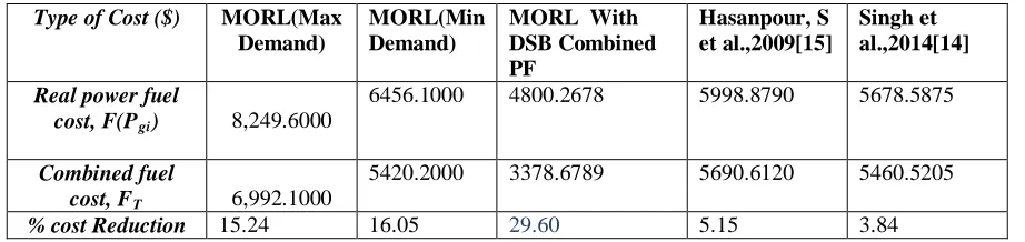
[15]($5690.6120) were found to be higher compared even to the DSB-MORL at minimum load($ 5420.2000) for the CRRED ,that is the MORL 15.24% 16.05 % better using the max and min approach respectively.The MORL with DSB Resulted into a far much reduced cost of $3378.6789 (29.6%) as compared to all other methods as losses involved have been optimized by DSB and further by MORL. The method provided an exhaustive search of the problem space with reduced number of iterations, reduced fuel cost and a better voltage profile.

Table 11.0: Comparison of proposed method with methods

Type of Cost ($) MORL(Max Demand)

MORL(Min Demand)

MORL With DSB Combined PF Hasanpour, S et al.,2009[15] Singh et al.,2014[14]

Real power fuel

cost, F(Pgi) 8,249.6000

6456.1000 4800.2678 5998.8790 5678.5875

Combined fuel

cost, FT 6,992.1000

5420.2000 3378.6789 5690.6120 5460.5205

% cost Reduction 15.24 16.05 29.60 5.15 3.84

VI. CONCLUSION

DSB-MORL algorithm was successfully applied for the solution of CRRED. Power allocation was done among five generating units at optimum generating costs while taking into consideration the equality, inequality and the stochastic constraints. From the results and analysis done, CRRED of power was found to be cheaper by almost 0.95%(~$ 40/Hr)than when real dispatch of power only is considered. When network losses were optimized using the DSB and then RL applied for the CRRED, the cost was found to be even lower as compared to the pure RL. Reduced losses meant reduced cost due to the introduction of the renewable energy based reactive power. Dynamic reactive power results in improved reactive power management and improved voltage profile, hence reduced optimal cost. The DSB-MORL with Combined PF provided a feasible solution with fewer iterations as compared to the real power PF, reactive power PF and SSB. However, a better optimal cost can be achieved if more accurate cubic cost functions are used in modelling the CRRED. Lastly, increased practical application of the proposed DSB-MORL can be realized by showing the test results on IEEE 57 bus and IEEE 118 bus systems which are larger and more realistic.

ACKNOWLEDGEMENT

The authors gratefully acknowledge The Deans Committee Research Grant (DCRG) The University of Nairobi, for funding this research and the Department of Electrical and Information Engineering for providing facilities to carry out this research Work.

REFERENCES

[1] Lee, K.Y.; Park, Y.M.; Ortiz, J. L., "A United Approach to Optimal Real and Reactive Power Dispatch," Power Apparatus and Systems, IEEE Transactions on , Vol.PAS-104, No.5, pp.1147,1153, May 1985.

[2] Serrano, B. R.; Vargas, A., "Active-reactive power economic dispatch of very short term in competitive electric markets," Power Technology Proceedings, 2001 IEEE Porto, Vol.1, No.10 pp.6-8, 2001.

[3] Worawat Nakawiro et al “A Novel Optimization Algorithm for Optimal Reactive Power Dispatch: A Comparative Study” IEEE Transactions on Power Systems, Vol.1 pp. 1155-1161, 2011.

[4] R. Mallipeddi et al “Efficient constraint handling for optimal reactive power dispatch problems” Swarm and Evolutionary Computation Vol. 5, Pages 28-36, August 2012.

[5] Lopez, J.C.; Munoz, J.I.; Contreras, J.; Mantovani, J. R S, "Optimal reactive power dispatch using stochastic chance-constrained programming," Transmission and Distribution: Latin America Conference and Exposition (T&D-LA), 2012 Sixth IEEE/PES , Vol.3, pp.1-7, 3-5 Sept. 2012

[6] Q.H. Wu, Y.J. Cao, J.Y. Wen ”Optimal reactive power dispatch using an adaptive genetic algorithm” International Journal of Electrical power and energy systems Vol.20, Issue 8, Pages 563–569, November 1998.

[7] Yusuf Sonmez “Estimation of Fuel cost curve parameters for thermal power plants using the ABC Algorithm“ ,Turkish Journal Of Electrical Engineering and Computer Science ,Vol .21 pp. 1827-1841,2013

[8] K.M.S.Tong andM.Kleinberg, “A distributed slack bus model and its impact on distribution system application techniques,” in Proc. IEEE Int.Symp.CircuitsSyst. (ISCAS),vol.5, pp.4743–4746,May2005.

[9] S.TongandK.Miu, “A network-based distributed slack bus model for DGs in unbalanced power how studies, IEEETrans.PowerSyst” vol.20, no. 2, pp. 835–842, May 2005

[10] K. M. S. Tong, “Participation factor studies for distributed slack bus Models in three-phase distribution power flow analysis,”inProc.IEEE PESTransm.Distrib.Conf.Exhib.,2005/2006, pp.92–96,May 2006.

[11] S. Tong and K. Miu, “Slack bus modeling and cost analysis of distributed generator installations,” J. Energy Eng., vol. 133, no. 3, pp.111–120, 2007.

[13] E. A. Jasmin et al "Reinforcement Learning Approaches to Economic Dispatch Problem," Electrical Power and Energy Systems, Vol 33 ,pp 836-845, 2011 [14] Singh, H. P., Brar, Y. S., & Kothari, D. P., “Combined active and reactive power dispatch using Particle Swarm Optimization” Proceedings of Informing Science

& IT Education Conference (InSITE) 295-304, 2014.

[15] Hasanpour, S., Ghazi, R., & Javidi, M. H. “A new approach for cost allocation and reactive power pricing in a deregulated environment”. Electrical Engg.,91 (1), 27-34,2009

[16] Deksnys, R., & Staniulis, R., “Pricing of reactive power services”. Oil Shale Estonian Acad. Publ.,24, 363–376,2007.

[17] Baughman, M. L., & Siddiqi, S. N. “Real time pricing of reactive power: Theory and case study results”. IEEE Trans. Power Sys.,6, 23-29,1993. [18] Kahn, E., & Baldick, R. “ Reactive power is a cheap constraint”. The Energy Journal, 15, 191-201,1994.

[19] Muchayi. M., &. El-Hawary, M. E. “A summary of algorithms in reactive power pricing”. Electric Power and System Research, 21, 119-124,1999. [20] Hogan, W.(1993). “Markets in real electric networks require reactive prices”. The Energy Journal, 14(3), 171-200,1993.

[21] Niknam, T., Arabian, H., & Mirjafari, M. “Reactive power pricing in deregulated environments using novel search methods”. IEEE Proceedings of Third International Conference on Machine Learning and Cybemetics, Shanghai, pp. 4234–4240,2004

[22] Bialek, J.W.,&Kattuman, P.A. “Proportional sharing assumption in tracing methodology”. IEE Proceedings Generation Transmission and Distribution, 151(4), 526-532,2004.

[23] Chung, C.Y., Chung, T. S., Yu, C.W., & Lin, X.J. “Cost-based reactive power pricing with voltage security consideration in restructured power systems”. Electr Power Syst Res.,70, 85–92,2004.

[24] Moses Peter Musau, Nicodemus Odero Abungu, Cyrus Wabuge Wekesa. “Multi Objective Dynamic Economic Dispatch with Cubic Cost Functions”. International Journal of Energy and Power Engineering. Vol. 4, No. 3, pp. 153-167,2015

AUTHORS

First Author – Moses Peter Musau , Department of Electrical and Information Engineering, School of Engineering, The University of Nairobi, Nairobi, Kenya, Email: [email protected]

Second Author – Nicodemus Odero Abungu, Department of Electrical and Information Engineering, School of Engineering, The University of Nairobi, Nairobi, Kenya, Email: [email protected]