DYNAMIC SENSOR RELOCATION TECHNIQUE BASED LIGHT WEIGHT INTEGRATED PROTOCOL FOR WSN

565

DESIGN OF AIRFOIL USING

BACKPROPAGATION TRAINING WITH

PENALTY TERM

1_{K.Thinakaran,} 2_{Dr.R.Rajasekar}

1_{Associate Professor, Sri Venkateswara College of Engineering &} Technology, Thiruvallur

2_{Professor, Srinivasan Engineering College, Perambalur}

E-mail: [email protected], 2 [email protected]

ABSTRACT

Here, we investigate a method for the inverse design of airfoil sections using artificial neural networks (ANNs). The aerodynamic force coefficients corresponding to series of airfoil are stored in a database along with the airfoil coordinates. A feedforward neural network is created with input as a aerodynamic coefficient and the output as the airfoil coordinates. . In existing algorithm as an FNN training method has some limitation associated with local optimum and oscillation. In this paper new cost function is proposed for hidden layer separately. In the proposed algorithm the output layer is incorporated into to the cost function having linear and non linear error terms. The functional constraints penalty term at the hidden layer are incorporated into to the cost function having linear and nonlinear error terms. Results

indicate that optimally trained artificial neural networks may accurately predict airfoil

profile.

Keywords: Linear Error, Nonlinear Error, Steepest Descent Method, Airfoil Design, Neural Networks, Backpropagation, Penalty Term.

1. INTRODUCTION

In order to develop aircraft components and configurations, automated design procedures are needed. At present, there are two main approaches to the design of aircraft configurations. The first is direct optimization, where an aerodynamic object function, such as the pressure distribution is optimized computationally by gradually varying the design parameters, such as the surface geometry. The second is the inverse design methods. Here, a two dimensional airfoil profile is obtained for the given coefficient of lift (CL) and the coefficient of

drag(CD).

But the backpropagation takes long time to converge the computational effort can therefore be excessive. Some focused on better function and suitable learning rate and momentum (18-22). Details on the use of numerical optimization in aerodynamic design can be found in works by Hicks and other authors. (1-3). In inverse design

methods, the aim is to generate

geometry for airfoil. There are many

inverse techniques in use, for example,

hodo-graph methods for two

dimensional flows (4-6) and other two

dimensional formulations using panel

methods (7-8). The above

566 Han et al. proposed two modified constrained to obtain faster convergence (25). The additional cost terms of the first algorithm are selected based on the first order derivatives of the activation functions of the hidden neurons and second order derivatives of the activation of the output neurons. Second one are selected based on the second order derivatives of the activation functions of the hidden neurons and first order derivatives of activation functions of the output neurons.

The objective of this work is to show that artificial neural networks can be trained to design airfoil profiles. We have proposed new cost function by incorporating functional constraints proposed by Han et al and the cost function proposed by Abid et al(25). In the proposed algorithm the output layer is incorporated into to the cost function having linear and non linear error terms. The functional constraints penalty term at the hidden layer are incorporated into to the cost function having linear and nonlinear error terms. It converges faster than the non linear method. ANNs are able to perform even in the presence of noise in the data.

2.ANN TRAINING METHOD

Figure 1.Schematic Diagram for a Simple Neuron

Here, n_i is called the state or activation of the neuron i.g() is a general non linear function called variously the activation-function. The weight wij represents the strength of the

connection between neurons i and j. µi is the threshold value for neuron i, the general architecture of a two layer neural network with feed-forward connections and one hidden layer is shown in Figure3. The input layer is not included in the layer count because its nodes do not correspond to neural elements. The weighted sum of the inputs must reach the threshold value for the neuron to

transmit. One drawback associated with

neural networks is that it is normally very difficult to interpret the values of the connecting weights wij in terms of the task being implemented.

Neural networks offer a very powerful and general framework for representing nonlinear mappings from several input variables to several output variables. Since the goal is to produce a system which makes good predictions for new data. Training generally involves minimization of an appropriate error function defined with respect to the training set. Learning algorithms such as the back-propagation algorithm for feed-forward multilayer networks (16) help us to find such a set of weights by successive improvement from an arbitrary starting point.

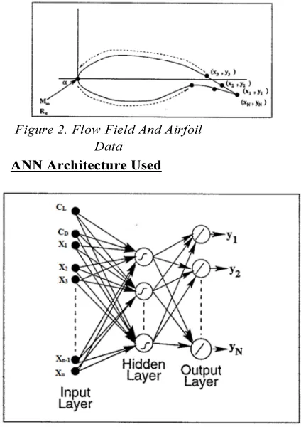
An airfoil profile can be described by a set of x- and y-coordinates, as illustrated in figure2.

Figure 2. Flow Field And Airfoil Data

ANN Architecture Used

Figure3. The Neural-Network Model Trained

To Predict Surface Y-Coordinates And Cl, Cd

567

The aerodynamic force coefficients

corresponding to series of airfoil are stored in a database along with the airfoil coordinates. A feedforward neural network is created with input as a aerodynamic coefficient and the output as the airfoil coordinates. This is then trained to predict the corresponding surface y-coordinates

We used the below sigmoidal activation function to generate the output.

షೣ

₍₁₎

For a neuron j at output layer L, the linear outputs given by Abid et al. is

_∑

(2)

Where wji is the weight connection

between the output neuron j and hidden neuron i. And is the output of neuron i at hidden layer H.

And the non linear output given by Abid et al. is

ష౫ౠై (3)

The non linear error is given by

e ₍₄₎

Where and respectively is desired and current output for jth unit in the Lth layer.

The linear error is given by e

₍₅₎

Where _{is defined as below}

(Inversing the o/p layer)

The learning function depends on the instantaneous value of the total error. As per the modified backpropagation by Abid et al, the new cost term to increase the convergence speed is defined as

(6 )

Where

λ

Now, this new cost term can be interpreted as below

Ep = (nonlinear error + Linear error)

To achieve low input and output mapping the error must be reduce by derivative of cost function When the value of becomes larger. So the proposed algorithm has penalty term defined by Jeong and Lee[24] at the hidden layer in addition with cost function having linear and non linear term, which is defined as follows

_ _ /_ ^′′ _"^

We have proposed new cost function for MBFC. This procedure, the dependence of the learning function is on the instantaneous value of the total error thereby leading to faster convergence.

MBFC

The new cost term to increase the convergence speed is defined as

1 2

1

2

_penalty

Ep =(nonlinear error+ Linear error -penalty)

Now, the weight update rule is derived

by applying the gradient descent method to Ep.

Hence we get weight update rule for output Layer L as

Δw ೛ _ೕ೔

Where is the network learning paramater

Δw - -

-

Δw -

- -

-

Δw ₍₇₎

Learning of the hidden Layer

And we get the weight update rule for the hidden layer H as

Δw ೛

_ೕ೔ - Penalty

Δw ೕಹ

_ೕ೔

ೕಹ

_ೕ೔ - Penalty

Δw ೕಹ

_{ೕ ೕ}ಹ

_ೕ೔

_-

Penalty

Δw _-

ಹ

_ಹ

₍₈₎

The network learning parameter µ is initialized, which plays an important role in minimizing the error. Then the network is trained with corresponding change of weight for both hidden and output layer. And the weight is determined by calculating linear, nonlinear error. Which play an important role in minimizing the error. Then the network is trained with new cost function.

Proposed Algorithm

In the Proposed Algorithm the network

learning parameter is first initialized. Here, the change of weight for output layer and hidden layer is determined using new cost function equation (7)and (8) respectively.

Step1: Initialize the parameter μ to some random values Step2: Assign Threshold value to a

fixed value based on the sigmoid function.

Step3: Calculate linear output using equation (2)

Step4: Calculate Non-Linear output using sigmoid function as in the equation (3)

Step5: Calculate the below values for output layer

Calculate weight change for output layer using the equation (7) Step6: Calculate the below values for

hidden layer

Calculate the weight change for hidden layer using the equation (8)

Step7: Calculate the mean square error Step8: If the mean square error value

is greater than threshold value, then the above steps from 3 to 7 is repeated Step9: If the mean square error value

is less than threshold value, then declare that the network is trained

3. RESULTS AND DISCUSSION

In our investigation of neural network models for inverse design, we found that satisfactory results were obtained by using a feedforward neural network with a penalty term in the hidden layer learning. In our case, it was found that twenty hidden nodes could adequately capture the nonlinear relationship between the airfoil profiles.

As mentioned previously we have a database comprised of 26 upper and lower-surface x and y coordinates, together with the corresponding coefficient of lift(CL)

and the coefficient of drag(CD). There were

1422 patterns in total. The main goal is

569

-0.50000 0.00000 0.50000 1.00000 1.50000 2.00000 2.50000 3.00000

0 10000 20000 30000

Convergence History

Convergence History with penalty Term

The network was trained to minimum error (using 1000 training patterns) on a test set (comprising 422 patterns) which was not used in the training process. The computed profiles show good agreement with the actual profiles. The new airfoil is tested again for the same flow conditions in XFoil tool to compare Cl, Cd.

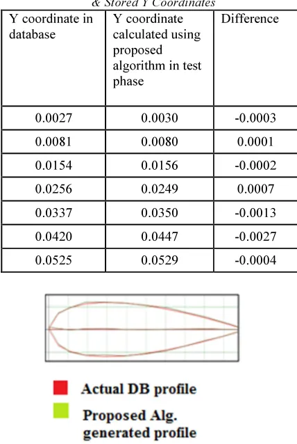
In Table I, we have given the values of stored y coordinates, the values of calculated y coordinates for a pattern and also the difference between these values. Just for sample, we have given 7 coordinates out of 26 coordinates for a pattern. From this table, we can say that the computed profiles generated during the test process show good agreement with the actual profiles.

Table I - Profile Comparison Between Calculated & Stored Y Coordinates

Y coordinate in database

Y coordinate calculated using proposed algorithm in test phase

Difference

0.0027 0.0030 -0.0003

0.0081 0.0080 0.0001

0.0154 0.0156 -0.0002

0.0256 0.0249 0.0007

0.0337 0.0350 -0.0013

0.0420 0.0447 -0.0027

0.0525 0.0529 -0.0004

Figure 4 – Airfoil Profile Comparison

This figure 4 is prepared using the profile stored in database and using the profile generated from the proposed algorithm during test phase. The red color airfoil is drawn using the profile namely naca0012 stored in database. The green color airfoil is drawn using profile naca0012 generated by proposed algorithm during test phase. From this figure, we can say that the computed profiles generated during the test process show good agreement with the stored database profiles.

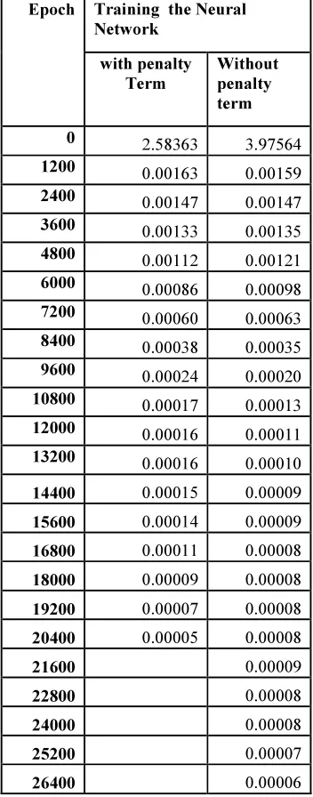
From figure4, we can say that the computed profiles generated during the test process show good agreement with the stored database profiles. Next we compute the convergence rate at training phase. To do this, we noted down the MSE error at each epoch and plotted it in the graph in Figure5. The blue line indicates the error. it is clear that our approach converges quickly and in this approach the error is less at the converging stage. It shows how the training decreases mean square Error (MSE) with the epoch. From this figure it is obvious that using penalty term increase the converges speed and without oscillation of learning.

Figure5. Convergence Of Trained Neural

Network.

approximately correct airfoil without

oscillation in learning. This proves that the proposed approach results in less error and takes less time to predict the airfoil for the given CL & CD.

Table Ii - Comparison Table

Epoch Training the Neural Network

with penalty Term

Without penalty term

0 _{2.58363 3.97564}

1200 _{0.00163 0.00159}

2400 _{0.00147 0.00147}

3600 _{0.00133 0.00135}

4800 _{0.00112 0.00121}

6000 _{0.00086 0.00098}

7200 _{0.00060 0.00063}

8400 _{0.00038 0.00035}

9600 _{0.00024 0.00020}

10800 _{0.00017 0.00013}

12000 _{0.00016 0.00011}

13200 _{0.00016 0.00010}

14400 0.00015 0.00009

15600 0.00014 0.00009

16800 0.00011 0.00008

18000 0.00009 0.00008

19200 0.00007 0.00008

20400 0.00005 0.00008

21600 0.00009

22800 0.00008

24000 0.00008

25200 0.00007

26400 0.00006

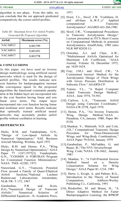
Figure6 contains the airfoils naca0012, naca0014 and naca1017 which are generated by proposed algorithm in test phase. From this figure, we can say that profile generated from proposed algorithm in test phase matches with that

of stored database profiles. Thus we observe that the adaptive learning rate approach generated comparatively the correct airfoil profiles

Figure6. Proposed Alg. Generated Airfoils

A measure of the accuracy of the results obtained can be inferred from examination of error which is defined as

/ !" 0/0 102344 0/∗ 100

571 algorithm in test phase. From this table, we can conclude that the our approach predicated comparatively the correct airfoil profiles.

Table III - Maximum Error For Airfoil Profiles Generated By Proposed Algorithm.

4. CONCLUSIONS

In this paper, we have used an inverse design methodology using artificial neural networks which is used for the design of airfoil profiles. The results indicate new cost function for backpropagation increase the convergence speed. In the proposed

algorithm the functional constraints penalty

term at the hidden layer are incorporated into to the cost function having linear and non linear error terms. The output layer incorporated into cost function having linear and nonlinear error terms. Results indicate

that optimally trained artificial neural

networks may accurately predict airfoil profile without oscillation in learning.

REFERENCES

[1]. Hicks, R.M. and Vanderplaats, G.N., "Design of Low-Speed Airfoils by Numerical Optimization," SAE Business Aircraft Meeting, Wichita, April 1975 [2]. Hicks, R.M. and Henne, P.A., "Wing

Design by Numerical Optimization," AIAA Paper 77 1247,1977[3]. Vanderplaats, G.N., "CONMIN A FORTRAN Program for Constrained Function Minimization," NASA TMX- 62282, 1973

[3]. Nieuwland, G.Y., "Transonic Potential Flow around a Family of Quasi-Elliptical Airfoil Sections,"National Luchten Ruimtevaar Laboratorium Amsterdam, NLR-TR- T.172, 1967

[4]. Garabedian, P.R. and Korn,

D.G.,"Numerical Design of Transonic Airfoils," Numerical Solution of Differential Equations - II, Academic Press,

1971

[5].Hoist, T.L., Sloof, J.W. Yoshihara, H. and all-haus Jr.,W.F.,z" Applied

computational Transonic

Aerodynamics" AGARD-AG-266,1982

[6].Sloof, J.W., "Computational Procedures in Transonic Aerodynamic Design," Lecture presented at ITCS Short Course on Computational Methods in potential Aerodynamics, Amalfi,Italy, 1982 (also NLR MP 82020 U)

[7].Ormsbee, A.I. and Chen, A.W., "Multielement Airfoils Optimized for Maximum Lift Coefficient, "AIAA Journal, Volume 10, December 1972, pp. 1620-1624.

[8].Fray, J.M.J. and Sloof, J.W., "A Constrained Inverse' Method for the Aerodynamic Design of Thick Wings with Given Pressure Distribution in Subsonic Flow," AGARD-CP.

[9].Tranen, T.L., "A Rapid Computer Aided Transonic Design Method," AIAA , June 1974, 74-501.

[10].Carlson, L.A., "Transonic Airfoil Design using Cartesian Coordinates," NASA-CR-2578, April 1976

[11].Henne, P.A., "An Inverse Transonic Wing Design Method,"AIAA , Pasadena, CA.,January 1980, Paper 80-0330.

[12].Shankar, V., Malmuth, N.D. and Cole, J.D.," Computational Transonic Design Procedure for Three-Dimensional Wings and Wing-Body Combinations," AIAA Paper 79-0344, January 1979

[13].Garabedian, P., McFadden, G. and Bauer, B.,"The NYU InverseSwept Wing Code,"NASA CR-3662, January 1983

[14].Shankar, V., "A Full-Potential Inverse

Method based on a Density

Linearization Scheme for Wing Design," AIAA Paper 81-1234, 1981

[15].Hertz, J., Krogh, A. and Palmer, R.G., Introduction to the Theory of Neural

Computation, Addison-Wesley

Publishing Co., California, 1991

[16].Riedmiller, M. and Braun, H., "A Direct Adaptive Method for Faster Backpropagation Learning: the RPROP

Airfoil Maximum error (%)

NACA0012 _0.001799

NACA0014 _0.001493

Algorithm," Proceedings of the IEEE

International Conference on Neural Networks, San Francisco, CA, March 28-April 1, 1993

[17].L.Behera, S. Kumar, A. Patnaik “On adaptive learning rate that guarantees convergence in feedforward networks”, IEEE Trans. Neural Networks 17, 1116-1125, (2006)

[18].R. A. Jacobs “Increased rates of convergence through learning rate adaptation”. Neural Networks 1, 295-307, (1988).

[19].G. D. Magoulas, V. P. Plagianakos, M. N. Vrahatis A. Van Ooyen, B.Nienhuis “Improving the convergence of the backpropagation algorithm”. Neural Networks. 5, 465-471,(1992).

[20].X. H. Yu, G. A. Chen, S. X. Cheng “Acceleration of backpropagation learning using optimized learning rate and momomentum”, Electron. Lett. 29, 1288-1289, (1993).

[21].T.Kathirvalavakumar, P. Thangavel “A modified backpropagation training algorithm for feedforward neuralnetworks”, Neural Processing Letters 23, 111-119, (2006).

[22].S. Abid, F. Fnaiech, M. Najim “A fast feedforward training algorithm using a modified form of the standard backpropagation algorithm”. IEEE Trans. Neural Networks 12, 424-430, (2001).

[23].R. Battiti “First and second order methods for learning: Between steepest descent and Newton’s method”, Neural Computation 4, 141-166, (1992).

[24].S. Y. Jeong, S. Y. Lee “Adaptive learning algorithms to incorporate additional functional constraints into neural networks”, Neuro computing 35, 73-90, (2000).

[25].F. Han, Q. H. Ling, D. S. Huang “Modified constrained learning algorithms incorporating additional functional constraints into neural networks”, Information Sciences 178, 907-919, (2008).

[26]. K. Levenberg, “A method for the solution of certain non-linear problems in least squares”,

Quarterly of Applied Mathematics 2, 164-168,