ONLINE DRIVING STATES MONITORING USING FUSION
OF MULTI-SENSOR INFORMATION
1, 2JIE MA, 1, 2XINPING YAN, 1, 2DUANFENG CHU, 1, 2YI HE
1Engineeing Research Center of Transportation Safety (Ministry of Education),Wuhan University of
Technology, Wuhan 430063, Hubei, China
2
Intelligent Transport System Research Center, Wuhan University of Technology,
Wuhan 430063, Hubei, China
ABSTRACT
In this paper, an online methodology for the detection of unsafe driving states while driving is presented. The detection is based on the multi-sensor approaches, including gyrometer, accelerometer, radar, video and so on. Various information comes from both the ego vehicle and its surroundings are fused to gain a comprehensive understanding of driving situations. Using subspace modeling techniques, we propose an unsupervised learning algorithm to perform the unsafe states detection. The feature space are decomposed into the normal and anomalous subspace, where the normal space are assumed as the major components of the driving patterns, and significant deviations from the modeled normal subspace are signaled as unsafe states. In addition, the algorithm works in a real-time way incorporating a implementation of sliding window, which enable the method to adapt over time to address changes in the new emerged driving situations. We have implemented our algorithm with a prototype system installed in a transit bus, validations are performed in real driving situations. Our experimental results demonstrate the effectiveness of the approach on forward risk predication. We gain a timely predication while with a low false positive when there occurs conflicts between the ego vehicle and front vehicles.
Keywords: Multi-sensor Fusion, Driving States Monitoring, Subspace Modeling
1. INTRODUCTION
Car accidents happen all the time and as a result of which people lose their lives, but the person behind the wheel tend not to consider it as such. Vehicle drivers are not always aware of all the dangerous conditions that are experienced while operating an automobile. A large number of fatalities occurring during car driving could be avoided if the right monitoring system was put in place. Due to recent advances in sensing technologies, vehicles are now equipped with multiple sensors, which broadens the awareness of the driver with significantly better information about their surrounding environment and the road ahead. In particular, sensor measurements can be integrated to detect unsafe driving states which can largely save drivers from exposure to dangerous situations. The present study will then focus on investigating the possibility to establish a new approach for online driving states monitoring using multiple sensors.
Research and development has actively been carried out for the past few decades, with the goal
because electrodes must be attached to the driver’s body. To develop nonintrusive driving safety monitoring systems, visual features extracted from face images are used to model the driver's state [5~7]. Two clues of interest have been explored, the first is the mean level of eye opening as an indicator of fatigue, the other is the movement of the head which could be an indicator for both fatigue and stress. Since the limitations of current computer vision techniques and the variations of driving environment, the visual features of eye opening and head movement cannot always be acquired accurately or reliably. Putting such monitoring systems in practice could make the estimation of drivers state less effective compared to experimental settings.
In practice, driving is a complex task involving a great amount of interaction among the driver, vehicle and environment. Drivers regularly share their attention among operating the vehicle, monitoring traffic and nearby obstacles, the complexity of the task and uncertainty of the driving environment make driving a very dangerous task. Therefore, it is not really a practical way to determine the driving safety just considering the driver's physiological or physical factors. More effective way to establish a driving safety monitoring system can be gained using other nonintrusive sensor data, including vehicle’s dynamic parameters, such as lateral positions, accelerations/decelerations, steering wheel movements, and environmental condition parameters, such as lane-marker recognition [8] and road-obstacle detection [9]. The challenge is to fuse these parameters to properly measure the safe/danger level for various driving situations. Accordingly, the interest of our work is concentrated on modeling these parameters rather than learning the driver's physiological or physical features.
By utilizing the technology of pattern recognition, data mining, data acquisition and system engineering, many studies were carried out in order to detect unsafe driving patterns. A set of research concentrates on developing incident detection system for automatic recognition of incidents, accidents and other road events requiring emergency responses. The focus is on learning probe vehicles data and the traffic data using inference method, such as Bayesian inference, Dempster-Shafer inference, and voting logic [10, 11]. However, these systems always need to be supplied with enough inference rules, which make it difficult to define a comprehensive set rules to cover all kinds of risky situations. Besides, these
systems often work remotely in a traffic management center, they cannot provide a real-time service to warn individual drivers with their respective driving situation. The ever-increasing computational capacity of mobile devices presents an opportunity for the knowledge discovery techniques in applications of the driving safety monitoring. The predominant approach is to use static classifiers such as support vector machines (SVMs) [3, 12]. A promising approach can be found in [13], where SVMs were applied to detect driver distraction using data captured under real traffic conditions. In [14], Hidden Markov Models (HMM) were used to create models of driving maneuvers, such as passing, switching lanes and starting and stopping, where the potentially dangerous move of a car could be predicted. Similar approaches toward driver states estimation that model contextual information via neural networks can also be found in [15]. However, several limitations deteriorate the applicability of the reported approaches. Fist, these systems are usually limited to very specific scenarios, such as driving under the influence of fatigue, they cannot identify more general dangerous driving patterns. Second, most of these reported works utilized supervised learning techniques to identify driving states. It is a really tough task to collect sufficient samples to train the learning systems, where calibrating the samples to clearly discriminate the safe and unsafe driving states is usually impossible. Third, the supervised learning or classificatory approaches lack the online capacity to adapt to the variations of driving environments and the instantaneous changes of driving states.
The main contributions of this work can be briefly described through the following points.
1) We propose a general framework for monitoring driving states. In this framework, multi-sensor approaches and fusion of data from both the ego vehicle and its surroundings are used to gain complimentary information, which results in a comprehensive understanding of driving situations.
2) Using subspace modeling techniques, an algorithm for unsafe driving states predication is presented. It is an unsupervised learning method, and there is no need to specify a model for safe or unsafe driving patterns, so that the data training and labeling issue can be avoided.
The rest of this paper is organized as follows. Section 2 gives an overview about the complete framework and the sensor integration. The details of the proposed detection algorithm are described in Section 3, Section 4 shows validation results. Conclusions are drawn in Section 5.
2. SYSTEM FRAMEWORK
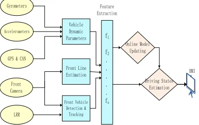
Driving states monitoring is concerned with the problem of estimating the motion of a vehicle and the changes of its surroundings. It focus on not only the current situation of vehicle, but also the future situation by predicting the potential dangerous possibility. In this framework, sensor fusion allows the system to obtain real-time information about vehicle dynamics and road environment, the resulting estimate is in some sense better than it would be if the sensors were used individually. Furthermore, the driving states estimation may in some cases only be possible to obtain by using data from different types of sensors. As shown in Figure 1 on the basis of various factors, an integrated driving states monitoring framework is introduced.
Front Line Estimation
Front Vehicle Detection &
Tracking Accelerometers
GPS & CAN
Vehicle Dynamic Parameters
Front Camera
LRR Gyrometers
f1
f2
. . . . . fn
Feature Extraction
Driving States Estimation
HMI Online Model
[image:3.612.92.294.380.507.2]Updating
Figure 1: Overall Architecture Of Our Framework
The framework consists of several elements that have different functionalities and carry out different roles in the overall design. The deployed sensors can be divided into two subgroups; there are internal sensors measuring the vehicle dynamic parameters, external sensor measuring the objects surrounding the vehicle. Internal sensors are referred to as proprioceptive sensors, including gyrometer, primarily measuring the yaw rate about
the vehicle’s vertical axis, and accelerometer, measuring the longitudinal and lateral acceleration of the vehicle. The velocity and heading of the vehicle is measured using GPS. The vehicle’s internal controller area network (CAN) bus provides other information about the vehicle operations, such as accelerograph and barking. External sensors are referred to as exteroceptive sensors, including a 77-GHz long-range radar (LRR) mounted at the front bumper, and a gray-scale camera installed on the front windshield.
knowledge about moving objects in the surrounding of the ego vehicle is gained by the long-range radar. Lane markings on the road surface are detected using the camera with a image processing procedure to extract the vehicle's lateral position relative to the two adjacent lanes. The radar and the camera complement each other very well, since the advantage of the radar is the disadvantage of the camera and vice versa. Therefore, the camera is also used to improve and stabilize the vehicle tracking. The information fusion of the two external sensors improves the reliability of the tracking algorithms and allows us to more accurately estimate the position of the perceived vehicles.
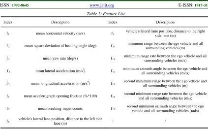
The raw perception parameter signals acquired from different sensors need to be synchronized. The sample frequencies of the raw signals range from 1 to 100 Hz. Thus, the data sequences are linearly interpolated to obtain a uniform frequency of 100 Hz before being synchronized. Consequently, A short time window (100 ms), denoted as a feature widow wf, is selected to apply on the raw data sequences, and the raw data points covered by this window are converted into one single feature vector
x. We denote each feature vector by xi = [f1,…,fn]
T
Table 1: Feature List
Index Description Index Description
f1 mean horizontal velocity (m/s) f9 vehicle's lateral lane position, distance to the right side lane (m)
f2 mean square deviation of heading angle (deg) f10
minimum range between the ego vehicle and all surrounding vehicles (m)
f3 mean yaw rate (deg/s) f11 minimum range rate between the ego vehicle and all surrounding vehicles (m/s)
f4 mean lateral acceleration (m/s2) f12 minimum azimuth angle between the ego vehicle and
all surrounding vehicles (rads)
f5 mean longitudinal acceleration (m/s2) f13
second minimum range between the ego vehicle and all surrounding vehicles (m)
f6 mean accelerograph opening fraction (%*100) f14
second minimum range rate between the ego vehicle and all surrounding vehicles (m/s)
f7 mean breaking input counts f15 second minimum azimuth angle between the ego vehicle and all surrounding vehicles (rads)
f8 vehicle's lateral lane position, distance to the left side
lane (m) / /
to update the predication model (see further details in the next section ). Finally, a decision for the dangerous driving state is passed as a warning to the driver through a human–machine interface (HMI).
3. METHOD
3.1 Problem Statement
As previously described in this paper, the vehicle dynamic parameters and its surrounding information have been transferred into the feature sequence which is a multidimensional time series data. These data contain various driving situations, but it is very difficult to make a clear distinction between the safe and unsafe driving states only focusing on every single feature point.
Figure 2: Data Segment Of A Feature Sequence
Figure 2 shows a data segment of one feature sequence containing partial components. The area of the red dashed rectangle in the diagram represents some dangerous events taking place,
which is manually identified using recorded video movies (We have installed two monitoring videos, one towards the drive, the other towards the outside of the vehicle, thus the driving process can be recorded for further offline analysis). The data fall into the rectangle can be labeled with unsafe state, and they occur within a very short time interval lasting just a few of feature windows. The main challenge of our task is to predicate the state for each feature vector evolving with the timeline.
[image:4.612.105.282.549.655.2]3.2 Subspace Modeling
PCA, also called Karhunen-Loeve transform, is a mathematically orthogonal linear transform that converts a set of observations of possibly correlated variables into a set of values of uncorrelated variables. The uncorrelated variables are the principal components. The first principal component catches the largest variance which means it has the strongest ability to cover the most information of original variables. The next components then each catches the maximum variance among the remaining orthogonal directions [16].
Considering the feature sequence X= [x1, ...,
xi, ..., xT], which in fact is a matrix with n×T entries, where n is the number of feature items (in our case
n=15), T is the length of the feature sequence, we will apply PCA on this matrix. First, we denote Y= XT and rewrite Y so that its columns have zero mean. Then we compute the covariance matrix S= YTY and perform the eigendecomposition of S yielding a set of n eigenvalues λj and eigenvectors
vj (1≤j≤n). We denote the n eigenvalues in decreasing order as λ1 ≥ ... ≥ λn and their corresponding and their corresponding eigenvectors as v1, v2 ,. . ., vn, where each eigenvector represent one principal component or principal axe. The first principal axe v1 is the vector that points in the direction of maximum variance in Y. Iteratively, once the leading k-1 principal axes have been determined, the k-th principal axe corresponds to the maximum variance of the residual.
To model the subspaces, the principal axes can be divided into two disjoint subsets, corresponding to normal and anomalous variation in feature space. Eigenvectors representing the set of normal axes span the normal subspace A, while eigenvectors representing the set of anomalous axes span the anomalous subspaceA. As discussed before, the normal subspace corresponding to the 'safe' part of the overall data takes the domination position, which means the normal subspace should capture most of the variance and the major profile of the overall data should be characterized by it. Therefore, determining the normal subspace is equal to answering what principal axes could be selected as normal axes to well capture the vast majority of the variance. Since the principal axes are arranged in order of contribution to the overall variance, we compute the proportions of eigenvalues to estimate the contribution for each principal axe by
1
n k
j j k
p =λ ∑ =λ (1)
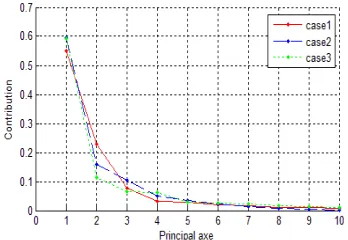
where the ratio pj indicates the contribution of the j -th principal axe. Figure 3 shows -the variance
[image:5.612.330.504.284.404.2]contribution of each principal axe for three cases of feature sequences. This plot reveals that more than 80 percent of total variance can be well accounted by 3 or 4 leading principal axes. Thus, we choose 3 or 4 leading principal axes as normal axes to construct the normal subspace if only these leading principal axes could capture at least 85 percent of total variance. In fact, the number of leading principal axes used for constructing the normal subspace should not too large, otherwise, it will cause some over-fitting problem that the modeling of normal subspace may be confused by some anomalous information, resulting in a wrong boundary between the normal and anomalous subspace.
Figure 3: Variance Contribution Of Each Principal Axe
3.3 Detection Algorithm
The main idea for detecting unsafe driving states from the multivariate feature sequence is based on the subspace decomposition. As we have constructed the normal subspace A , which is actually a matrix of size n×r where r denotes the number of normal axes, then each new generated vector x at any timestamp can be projected onto the space Aas
ˆ 1
( T ) T
x=A A A− A x (2)
such that ˆxcorresponds to the normal part of x . Since Ahas orthonormal collumns, we rewrite the eauation (2) as
ˆ T
x=AA x (3) And then the residual part, as well as the anomalous part, of x can be acquired as
x= −(1 AAT)x (4)
wherexis also regarded as performing projection of
xi onto the anomalous subspaceA, any changes in
there any significant deviation from the average level of the residual.
A typical statistic for detecting abnormal changes inxis the Squared Prediction Error (SPE)
2 (1 T) 2
SPE≡ x = −AA x (5)
An unsafe state can be identified by SPE>ε , whereεdenotes the threshold of SPE.
The average level of the residual part can be determined by calculating the Root Mean Square Deviation (RMSD) for a series of SPE data
2 1
{ }j T
i i j
SPE≡ x = ++ recorded historically.
2 2
1 1
( )
j T i
i j SPE
SPE T x E
δ + −
= + ∑
= (6)
where 2
1
1 i SPE
j T i j T
E = ∑= ++ x and then a δ driven
principal is used to form the threshold ε
ε=ESPE+θδSPE (7)
As such, the multiplier factor θ determines to what degree does a anomalous projectionxdeviate
from the average level of SPE can be regarded as a real anomaly or unsafe state.
Since the dynamic characteristics of driving situations, the variation in the structure of multivariate featur sequence over time is non-negligible. So it is unreasonable and impractical to examine the entire sensor data stream that accumulates over time. In practice, it can empirically be assumed that the unsafe states identification depends only on the sensor readings in the past T seconds. In other words, the subspace modeling can be carried out by analyzing the sensor data in a time window wT with the length of T
seconds, provided that there are no anomalies involving in the window. Usually, the time window
T
w is expected to work as a sliding window such that the model can accommodate itself dynamically to the changed driving situations. Figure 4 illustrates the working process of the proposed method.
Time axe
j+ T j+
1 j+2
j+ T + 1
j+ T+ C j+
C '
j+ C + 1
… …
… x
…
j+ T + 1
j+ T+ C
x
… … …
Subspace decomposition
Normal & anomalous subspace
Projection onto anomalous subspace
Threshold
ε
x
~
2≤
ε
x
~2
E
SPE SPE,
δ
Unsafe state
NO
YES
Model updating
1
2 3
4
5 j+
T
Feature sequence
T
w
C
w
As shown in the figure, the state predication for the oncoming feature data is based on the modeled information of a previous block of timewT. Another
time window wC is defined as a checking window
which determines the moving of wT and the model
updating. All data involved in wC should be processed to identify their corresponding states, and if none or only a very few of anomalies arise from
C
w , then the feature data contained in wCwill be added to the wT to update the model, and wT will
move to the end of wC, otherwise, the wC will be
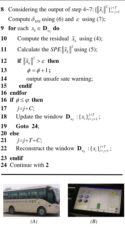
discarded and wT should be reconstructed using the new generated feature data. Algorithm 1 details the proposed method.
4. VALIDATION
To validate our approach in real driving conditions, we have implemented the algorithm with a prototype system installed in a transit bus, which is equipped with a variety of sensors. Figure 5 (a) shows a picture of the bus for experiments. The bus was put into service as a commercial coach, and several coach drivers were invited to drive the bus on a planned route under management of a highway transport company. Each trip lasted for more than 2 hours, and the driver was required to operate the vehicle as usual, no special instructions were given to the drivers. A experimenter, who is familiar with our system, was designated sitting beside the driver and was requested to observe the driving process and record some meaningful information, especially for dangerous events occurred in a trip. Figure 5 (b) shows a software interface of the system which can be used by the experimenter to make the recordings, and besides, it can output alarms with detected unsafe states.
Algorithm 1: Unsafe State Detection
1 Initialize: wT =30s, wC =10s,
T =300, C=100,θ =3, ϕ=10, φ=0; 2 Input feature data into the two windows:
1 1
:{ }
,
:{ }
T C
j T j T C
w
x
i i j wx
k k j T+ + +
= + = + +
D
D
;3 Subspace modeling for
T
w
D via PCA;
4 for each
T
i w
x ∈D do
5 Compute the residual xi using (4);
6 Calculate the SPE xi using (5); 7 endfor
8 Considering the output of step 4~7:{xi 2}ij T= ++j 1 ComputeδSPEusing (6) and ε using (7);
9 for each
C
k w
x ∈D do
10 Compute the residual xk using (4);
11 Calculate the SPE xk 2using (5); 12 if xk 2 >ε then
13 φ φ= +1;
14 output unsafe sate warning; 15 endif
16 endfor
16 if φ ϕ≤ then
17 j=j+C;
18 Update the window :{ } 1
T
j T
w xi i j
+ = +
D ;
19 Goto 24; 20 else
21 j=j+T+C;
22 Reconstruct the window :{ } 1
T
j T
w xi i j
+ = +
D ;
23 endif
24 Continue with 2
[image:7.612.312.519.88.464.2](A) (B)
Figure 5: The Developed Prototype System: (A) The Transit Bus Equipped With Multi-Sensors.
(B) Software Interface Of The System
real danger time points are actually identified and labeled by analyzing the logged recordings and image frames captured by the monitoring videos.
In Figure 6, we illustrate the effectiveness of our algorithm with 4 typical dangerous situations. For each case, a feature data segment spanning 40 seconds are used to explain the detection results, where dangerous events really occurred within the
later 10 seconds, and the time period of the previous 30 seconds was confirmed as safe time span which was used to perform the subspace modeling for the following detection. The upper half figure in each case shows time series plots of the original feature data x 2 over the 40 seconds periods.
(a) (b)
(C) (D) Figure 6: Predication Results For 4 Cases :
(A) Side Swiping During Lane Changing. (B) Rear-End Collision During Lane Changing. (C) Overtaking With High Speed. (D) Distraction Caused Rear-End Collision
In the lower half of each case we shows time series
plots of the residual part, namely the SPE x 2
,
over the same periods.As shown in the figures, the longer vertical red lines represent the identified real danger points tr, the shorter vertical dotted
blue lines represent the claimed danger time tp
of the checking window wC, it is common that
there exists continuous reported danger points tp. In addition, each dotted line of reported tp was appended a marker on its top, the circle shaped
markers represent true reports and the diamond shaped markers represent false reports, and besides, the lines labeled with tr are considered as the most dangerous point for each case. To make the
evaluation easier, the repeated reports of tp within one same checking window are counted as only one unsafe predication, and thus the statistics of true positives and false positives is just counting the numbers of checking windows which were labeled with safe or unsafe states. Simultaneously, we let the third time repeated report of tp be the unsafe predication point for that corresponding checking window, and it was marked in the figure with a longer vertical dotted blue line. This means that three continuously repeated reports of tp is the minimum for one time unsafe predication, and each checking window owns at most one unsafe predication. As such, some false detected points can be ignored by the system if these points cannot repeat themselves at least three times, which can reduce the false positives. More explaining about the four predicated dangerous situations will be described as follows.
Figure 6 (a) gives one kind of dangerous situation that the risk occurred during the vehicle's lane changing. The bus used for experiments was travelling on a three-lanes road, the bus driver was preparing to change from the left side lane into the middle lane, while a car in the right side lane was switching into the middle lane as well almost side swiping the bus. The bus driver changes back into the left side lane to avoid being hit. The risk duration is less than 5 seconds, and the unsafe predication was generated about 2 seconds earlier than the identified real danger time, which let the driver have time to make an appropriate response. The situation involved in case (b) is similar to case (a), it is also a lane changing caused risk. The bus driver changed from a left side lane into a middle lane and was continuing to change into another right side lane, while a car diving in the right side lane and in the front of the bus was beginning to decrease its speed, and then the bus driver steered a little to the left and slowed down his speed to avoid rear-end collision with the front car. Different from the previous case, the duration of this case takes a little more time, about 10 seconds, which provide us more time to make an unsafe predication. The predication time was advanced by 8 seconds comparing with the real danger time. In case (c), the ego bus driver was trying to overtake a van that was driving a bit more slowly than the bus, the bus driver made an emergent acceleration
and bypassed the van with a very high speed. Although no danger happened there, the process of this case is considered to be high risk since overtaking with high speed may cause some unpredictable crashes with other nearby vehicles. For this reason, the system also conveyed a timely alarm. The cause of case (d) has something to do with the bus driver. The driver was distracted by his mobile phone and did not notice a braking of the lead vehicle, when approaching too closely the bus driver applied his brakes to avoid hitting the lead vehicle. As indicated in the four cases, usually it quite difficult to see the effects of dangerous
events on the original feature data x2 as a whole, but the projection of the original feature data onto the residual subspace effectively captures the anomalous components while capturing little normal components, and so makes the unsafe driving states detection much easier. Among the 8 false reports in the 4 cases, only one false report was finally raised while others were all neglected. Based on our overall analysis of experimental results for all risks, the proposed method shows a good performance, true positive being 83.7% and false positive being 5.3%, on forward risk predication, such as side swiping and rear-end collision with front vehicles resulting from various causes, including lane changing, overtaking, distraction and so on. However, we cannot deal well with some other risky situations such as backward collisions coming from following vehicles or rear lateral directions. Besides, the average predication time for fast approaching risk, such as case (a) and (d), is 2~3 seconds ahead of the real danger points, and for slow approaching risk, such as case (b) and (c), the average time can be 6~8 seconds.
5. CONCLUSION
normal space corresponding to the major components of the overall data, anomalies that deviate significantly from the modeled normal subspace are signaled as unsafe states. Futhermore, the mechnism using sliding window makes it possible for our method to dynamically learn new information originated from the changed driving situations. Our experimental results demonstrate the effectiveness of the approach on forward risk predication. Our ongoing work is centered on employing more sensor techniques to extend the methodology proposed here to more risky situations, especially for predication of backward collisions.
ACKNOWLEDGEMENTS
This work is supported by the National Natural Science Foundation of China (No.61174173, No.61203236, NO.51105286) and by the National High Technology Research and Development Program of China (863 Program) (No. 2009AA11Z213).
REFERENCES:
[1] C.L. Lisetti, F. Nasoz, “Using noninvasive wearable computers to recognize human emotions from physiological signals”,
EURASIP Journal on Advances in Signal Processing, Vol. 2004, No. 1, 2004, pp. 1672-1687.
[2] P. Rani, J. Sims, R. Brackin, and M. Sarkar,
“Online stress detection using
psychophysiological signals for implicit human-robot cooperation”, Robotica, Vol. 20, No. 6, 2002, pp. 673-685.
[3] J. Zhai, A. Barreto, “Stress detection in computer users based on digital signal processing of noninvasive physiological variables”, Proceedings of 28th Annual International Conference of the IEEE EMBS, Aug. 2006, pp. 1355-1358.
[4] R. Bittner, P. Smrcka, M. Pavelka, P. Vysok, and L. Pousek, “Fatigue indicators of drowsy drivers based on analysis of physiological signals”, Proceedings of the 2nd International Symposium on Medical Data Analysis, Oct. 2001, pp. 62-68.
[5] Q. Ji, Z. Zhu, and P. Lan, “Real time nonintrusive monitoring and prediction of driver fatigue”, IEEE Transactions on Vehicular Technology, Vol. 53, No. 4, 2004, pp. 1052-1068.
[6] M.H. Sigari, “Driver Hypo-Vigilance Detection based on Eyelid Behavior”, Proceedings of the 7th International Conference on Advances in Pattern Recognition, Feb. 2009, pp.426-429. [7] J. Batista, “A Drowsiness and Point of
Attention Monitoring System for Driver Vigilance”, Proceedings of IEEE Intelligent Transportation Systems Conference, Sept. 2007, pp. 702-708.
[8] R. Schubert, G. Wanielik, M. Hopfeld, and K. Schulze, “Lane recognition using a high-resolution camera system”, Proceedings of Advanced Microsystems for Automotive Applications, 2009, pp. 209-227.
[9] S. Cherng, C.Y. Fang, C.P. Chen, and S.W. Chen, “Critical motion detection of nearby moving vehicles in a vision-based driver-assistance system”, IEEE Transactions on Intelligent Transportation Systems, vol. 10, no. 1, Mar. 2009, pp. 70-82.
[10] N.E. Thomas, "Multi-sensor multivariate and multiclass incident detection system for arterial streets", Proceedings of the 16th International Symposium on Transportation and Traffic theory, 1996, pp. 315-340.
[11] S.C. Byun, D.B. Choi, B.H. Ahn, H. Ko, "Traffic incident detection using evidential reasoning-based data fusion", Proceedings of the 6th World Congress on ITS, Nov. 1999. [12] Y. Liang, M. L. Reyes, and J.D. Lee,
“Real-time detection of driver cognitive distraction using support vector machines”, IEEE Transactions on Intelligent Transportation Systems, vol. 8, no. 2, Jun. 2007, pp. 340-350. [13] M. H. Kutila, M. Jokela, T. Mäkinen, J.
Viitanen, G. Markkula, and T.W. Victor, “Driver cognitive distraction detection: Feature estimation and implementation”, Proceedings of the Institution of Mechanical Engineers - Part D, Sept. 2007, pp. 1027-1040.
[14] N. Oliver, A.P. Pentland, "Graphical Models for Driver Behavior Recognition in a SmartCar", Proceedings of IEEE intelligent vehicles symposium, Oct. 2000, pp. 7-12.
[15] T.D. Orazio, M. Leo, C. Guaragnella, and A. Distante, “A visual approach for driver inattention detection”, Pattern Recognition, vol. 40, no. 8, Aug. 2007, pp. 2341-2355.
[16] Doam X. Tien, Khiang-Wee Lim, and Liu Jun, "Comparative Study of PCA Approaches in Process Monitoring and Fault Detection",