AN EFFICIENT SUPER PEER SELECTION ALGORITHM FOR PEER TO PEER (P2P) LIVE STREAMING NETWORK

ENERGY REALIZATION FISHEYE STATE ROUTING

ALGORITHM FOR MOBILE ADHOC NETWORKS

1_{R. HEMALATHA,} 2_{Dr.R.S.BHUVANESWARAN}

1_{Research Scholar, Ramanujan Computing Centre, Anna University, Chennai, INDIA}

2_{Associate Professor, Ramanujan Computing Centre, Anna University, Chennai, INDIA}

E-mail: [email protected], [email protected]

ABSTRACT

Energy consumption is prominent and critical issue faced by mobile adhoc network. Maximum energy is

consumed when the data is send from one node to another node. Therefore energy efficient routing

mechanisms are required. In this paper, a routing scheme based on the fisheye state routing with two groups of selection of nodes are achieved. One group of nodes having maximum energy and another group of nodes having minimum energy. According to the number of packet received the particular group of nodes are selected to send the data from the source to the sink. In this way the energy is utilized efficiently in the data sending process. This gives the reduction in the overall energy consumption of the network. This scheme is named as Energy-Realization Fisheye State Routing (FSR). The parameters of FSR and ER-FSR are compared. Results show that the proposed algorithm effectively utilizes the energy to all nodes.

For comparison various parameters like end-to-end delay average, Jitter and throughput have been considered.

Keywords: Fish eye state routing, Mobile ad-hoc network, Energy, Throughput, Jitter, End to end delay

1.

As the wireless and embedded computing technologies continue to advance, increasing numbers of small size and high performance computing and communication devices will be capable of tether less communications and ad hoc wireless networking. Mobile Ad hoc Network (MANET) is a collection of mobile nodes change their position randomly as they are free to move anywhere. Each time the mobility of node causes to change in the topology and hence the links between the two nodes are always changing in a random manner. In MANET, all mobile nodes will get their energy from batteries, which is a limited resource, whatever energy the mobile nodes have, it has to be used very efficiently. Also the nodes of a MANET may stop transmitting or receiving or both, also even receiving requires power for arbitrary time periods and the routing protocol should be able to accommodate such sleep periods without overly adverse consequences. There are many routing protocols and mobility models available for Mobile Ad Hoc Networks [1]-[6] Mobile Ad hoc networks are generally composed by a large number of mobiles nodes, forming a large network without an

resources (e.g., bandwidth and power) make routing in ad hoc networks extremely challenging. To prefer the energy efficiency in mobile ad hoc networks, it is necessary to model the node energy consumption. Various proposed protocols in these complex networks that aim to reduce energy consumption [7],[8] or achieve self-configuration and self-organization. In this work, a new routing scheme called Energy-Realization Fisheye State Routing is introduced for Mobile Adhoc Network. Further, how the available energy is utilized in a efficient way among the nodes is explained.

2.

node detects a topology change. In FSR, link state packets are not flooded. Instead, nodes maintain a link state table based on the up-to-date information received from neighboring nodes, and periodically exchange it with their local neighbors only (no flooding). Through this exchange process, the table entries with larger sequence numbers replace the ones with smaller sequence numbers.FSR reduces the routing update overhead in large networks. When network size grows large, the update message could consume considerable amount of bandwidth, which depends on the update period. In order to reduce the size of update messages without seriously affecting routing accuracy, FSR uses the Fisheye technique. Further, FSR minimized the consumed bandwidth as the link state update packets that are exchanged only among neighboring nodes and it manages to reduce the message size of the topology information due to removal of topology information concerned far-away nodes. Sending data to all neighboring nodes is the wasted one. This leads to increased energy consumption in the network.

3. ENERGY REALIZATION FISHEYE STATE ROUTING (ER-FSR)

To avoid the problem of sending information to all neighboring nodes, only selected group of neighboring nodes having maximum energy or minimum energy are engaged to transmit the data. Maximum energy node or minimum energy nodes are selected depends upon the number of packets arrived. Among these selected neighboring nodes having maximum energy or minimum energy, the routing preference is given to shortest path node only to send the data. In this network, the source node is a variable one. The intermediate nodes can act like a source node and only one sink node is present in the network. Here there are two separate paths to reach the sink node. One path is established via maximum energy nodes or another path is established via minimum energy nodes. When maximum number of packets arrived, the minimum energy nodes automatically discarded and only the maximum energy nodes are engaged to receive the data. The information about the neighboring nodes is available in table on each node. This mechanism ensures that the energy is saved by sending the messages to the selected group of nodes and all the energy is not wasted throughout the network and the routing is done efficiently.

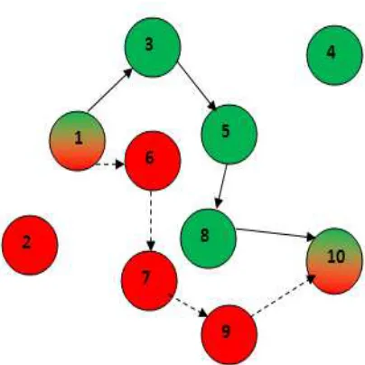
Fig1, shows the topology representation in ER-FSR. There are ten nodes with their respective energy levels at an instant of time is shown. Node ‘1’ acts as source node and node‘10’ acts as sink node. Steps to select a route in this network are:

Step 1: Assume at one instant of time more number of packets arrived at the source node 1. Node ‘1’ searches its one hop neighbors. From the one hop neighbors {2, 3, 6, 7}; node 2, 6 and 7 are not belong to the same group because these nodes are having minimum amount of energy. Hence node 3, having the maximum energy and hence it is eligible to accept the data.

Step 2: Now node 3 act as a source node now. The neighboring nodes are {4, 5, 6}. In this, node 6 is not belong to this group. Node 5 and node 6 are eligible to receive the data. In these two nodes preference is given to node 5 because as it establish shortest path. In that way the next hop is selected. Here node 5 and node 6 are having the same maximum energy but there distance is considered to send the data.

Step 3: The process of step 2 is followed to have the next hop to forward the data. Finally the data is received by the sink node 10. Hence the established path is 1-3-5-8-10.

3.1. ER-FSR path selection algorithm

4.

OFROUTING PROTOCOL

To evaluate the performance of routing protocols three different quantitative metrics to compare the performance of FSR and ER-FSR.

4.1.Average End-to-End Delay

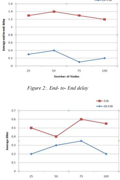
Average End-to-End delay is a metrics used to measure the performance with time taken by a pack to travel across a network from a source node to the destination node.Fig.1 shows the simulation results of average end to end delay with number of

nodes.

It is noticed that the delay for FSR

is

seconds while for ER-FSR it is below 0.5seconds. Further the presence of routing information is made available to the selected neighboring nodes only and this leads to average lower end-to-end delay only. The ER-FSR demonstrate lower delay than SR because of short time in discovering the route for selected nodes.

4.2. Average Jitter

Average jitter is a performance characteristics used to measure deviation from true periodicity eventually of inactivity in packet across a specific network.When a network is stabilized with constant

latency will have no jitter. Due to data congestion or route changes can cause jitter. From Fig.2, it is noticed that the ER-FSR show the better performance compared to FSR in terms of average jitter. ER-FSR has less jittering because it has one to one relaying technique for the selected neighboring nodes to provide optimal routes in terms of number of hops.

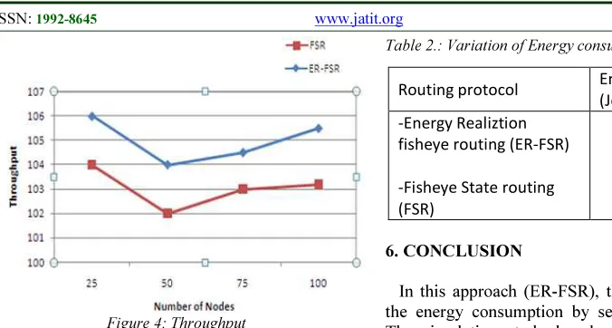
4.3. Throughput

The throughput is defined as the total amount of data a receiver receives from the sender divided by the time it takes for the receiver to get the last packet. Throughput is measured using number of bits of packet received per unit time. Normally throughput is measured as bits per sec.Fig.3 shows the simulation results for throughput for various number of nodes. ER-FSR show better performance than FSR because it can adjust dynamically according to the topology changes and gives better route than FSR.

Figure 2:. End- to- End delay

Figure 3: Average jitter

// ListN : Neighbor List // M1: Max threshold node

// M₂: Min threshold node // D: Destination Node 1.If find(ListN,D) NexthopD Return Endif

2.For(i0 to length(ListN))do D(n)=Energy(n)

ListN[i].dist = dist(ListN[i],D) Endfor

3. Find ‘v’ ,such that D(v)~=Max Threshold 4. M1 ‘v’

5. Find ‘w’ ,such that D(w)~=MinThreshold 6. M2 ‘w’

Figure 4: Throughput

5

Simulation experiment is set up using QualNet 5.0 network simulator [9]. Over an area of about 1000 x 1000 m2, a total of 100 nodes are deployed. Each node is made mobile by varying its speed while the sink node is kept static throughout the simulation. The ad hoc nodes generate CBR traffic towards the sink node at varying intervals of time. The mobility of the nodes with a pause time of 5s seconds is considered. Table 1 shows the other simulation parameters details. Effect of the changing mobility of the data gathering nodes on the network throughput, end-to-end delay and average jitter has been analysed. Effect of the changing mobility of the data gathering nodes on the network throughput, end-to-end delay and average jitter has been analysed. All the other simulations parameters are listed in Table 1 along with their values

Table 1:. Simulation parameters

Table 2.: Variation of Energy consumption

6. CONCLUSION

In this approach (ER-FSR), the aim is to reduce the energy consumption by selective nodes only. The simulation study has been conducted using network simulator QualNet 5.0 for the performance comparison of FSR. The simulation results shows that the Energy-Realization Fisheye Routing (ER-FSR) performs better for various number of nodes . The overall energy consumption of the network has decreased to almost 15%, ensuring longer network lifetime and at the same time ER-FSR provides better results than FSR in terms of average end-to-end delay, throughput and average jitter values. Thus this protocol is the best suited one compared with Fisheye routing protocol for the applications in which the network lifetime and efficient delivery of packets among nodes.

In future, the ER-FSR can be modified further to generate low control overhead by incorporating some optimization techniques like swarm intelligence.Also, real time environment can be used to study the actual behaviour of this protocol.

REFRENCES:

[1] Guangyu Pei; Gerla, M.; Tsu-Wei Chen; “Fisheye state routing: a routing scheme for ad hoc wireless networks,” IEEE International

Conference on Communications, 2000.

[2] D. Maltz, Y. Hu, “The Dynamic Source Routing Protocol for Mobile Ad Hoc Networks”,Internet

Draft,Available:http://www.ietf.org/internetdra fts/draft-ietf-manet-dsr-10.txt, July 2004. [3] A. Boukerche, “Performance evaluation of

routing protocols for ad hoc wireless networks”

Mobile Networks and Applications, Vol.9, No.

4, pp. 333-342, 2004.

[4] G. Fang, L. Yuan, Z. Qingshun, and L. Chunli, “Simulation and analysis for the performance of the mobile ad hoc network routing protocols”, The Eighth International Conference on Electronic Measurement and Instruments, IEEE Xplore, 2007.

Parameter Value

-Area of simulation -Number of nodes -Simulation time -Physical/MAC layer protocol

- -Routing protocol -Battery model -Energy model -Transmission power -Minimum velocity -Maximum velocity -Traffic type

-Number of connections -Source ID

-Destination ID -Start/End time

1000 x 1000m2 100 500 seconds 802.15.4 FSR/ER-FSR Linear micaZ 3dBm 10ms 20ms CBR 120 variable 1(sink node) variable

Routing protocol Energy Consumption

(Joule (mA h) -Energy Realiztion

fisheye routing (ER-FSR)

-Fisheye State routing (FSR)

2.55

[5] T. Camp, J. Boleng and V. Davies, “A survey of mobility models for ad hoc network research”, Wireless Communications and

Mobile Computing, Vol. 2, Issue 5,

pp.483-502, Aug 2002.

[6] Jardosh A, Belding-Royer EM, Almeroth KC, Suri S. “Towards realistic mobility models for mobile ad-hoc networks”. In: Proceedings of the 9th annual international conference on

mobile computing and networking

(MobiCom’03); September 14–19, 2003. pp.

217–29.

[7] L.Zhanjun, W. Rui, L. Qilie, L. Yun, C. Qianbin, and W. Ping, “An energy-constrained routing protocol for mobile ad hoc networks”,

International Conference on Communication Software and Networks, IEEE Computer Society,2009.

[8] V. Kanakaris, D. Ndzi and D. Azzi, “Ad-hoc networks energy consumption: A review of the ad hoc routing protocols”,Journal of

Engineering and Technology, review 3, pp.

162-167, 2010.