An Inventory Model for Deteriorating Items with
Exponential Declining Demand and Time-Varying
Holding Cost
Bhanu Priya Dash1, Trailokyanath Singh2, Hadibandhu Pattnayak3 1
Department of Mathematics, Kamala Neheru Womens College, Bhubaneswar, India 2
Department of Mathematics, C. V. Raman College of Engineering, Bhubaneswar, India 3
Department of Mathematics, KIIT University, Bhubaneswar, India Email: [email protected]
Received November 5, 2013; revised December 5, 2013; accepted December 12,2013
Copyright © 2014 Bhanu Priya Dash et al. This is an open access article distributed under the Creative Commons Attribution Li-cense, which permits unrestricted use, distribution, and reproduction in any medium, provided the original work is properly cited. In accordance of the Creative Commons Attribution License all Copyrights © 2014 are reserved for SCIRP and the owner of the intel-lectual property Bhanu Priya Dash et al. All Copyright © 2014 are guarded by law and by SCIRP as a guardian.
ABSTRACT
In the present paper, a total optimal cost of an inventory model with exponential declining demand and constant deterioration is considered. The time-varying holding cost is a linear function of time. Shortages are not allowed. The items (like food grains, fashion apparels and electronic equipments) have fixed shelf-life which decreases with time during the end of the season. A numerical example is presented to demonstrate the model and the sen-sitivity analysis of various parameters is carried out.
KEYWORDS
Constant Deterioration; Exponential Declining Demand; Inventory; Time Dependent Holding Cost
1. Introduction
The main objective of the proposed model is to develop an inventory model for a deteriorating item having a time-dependent exponential declining demand rate and time-varying holding cost. The literature review of the present paper is discussed as follows:
Generally, deteriorating items refer to the items that become damaged, decayed, spoiled, lost of utility or lost of its marginal value, evaporative, devaluation, invalid, degradation and so on through time. The process of de- terioration is happened in two categories of items. The first category refers to the items that become damaged, spoiled, decayed, loss of utility, evaporative or expired through time like food grain, food stuffs, fruits, flowers, vegetables, films, medicines and so on, while the other category refers to the items that loss their parts or their total values through time because of the introduction of new technology or the alternatives like fashion and sea- sonal goods, electronic equipments, computer chips and mobile phones and so on. For the first category, the items have a short natural life cycle whereas in the second category, the items have a short market life. The lite- rature surveys by Raafat [1], Wee [2], Shah and Shah [3], Goyal and Giri [4] and Li et al. [5] discuss the up to date review on deteriorating inventory model.
Mishra et al. [13]. Chang and Dye [14] established an inventory model with time-varying demand and partial backlogging. On the basis of demand variations, Ouyang and Cheng [15] developed an inventory model for de- teriorating items with exponential declining demand and partial backlogging. Abad [16,17], Shah and Raykun- daliya [18] studied the case of partial backlogging in their inventory model. Singh and Pattnayak [19] also stu- died an inventory model for deteriorating items with linear demand, variable deterioration and partial backlog- ging. Tripathy and Mishra [20], Singh and Pattnayak [21,22], Amutha and Chandrasekaran [23] also studied an inventory model on deteriorating items. Usually, in inventory models, inventory holding cost and the demand rate are considered to be constant. But sometimes in reality, we may observe that inventory holding cost and demand rate for physical goods are time-independent. This paper examines an inventory model with linearly varying holding cost. The objective function is to minimize the total cost of an inventory system based on in- ventory holding cost, ordering cost and deterioration cost. In reality, the demand rate and the inventory holding cost for physical goods may be time-dependent. As time is an important factor in the inventory system, we con- sider that demand rate and inventory holding cost are time-dependent. We have developed an EOQ inventory model for deteriorating items with exponentially declining demand when the deterioration rate follows a con- stant rate with time-dependent linear holding cost and shortages are not allowed.
In the present paper, an effort has been made to analyze an EOQ model for deteriorating items by considering the time-dependent exponential declining demand rate and time-dependent linear inventory holding cost. Short- ages are not allowed. The proposed model is based on the inventory items like fashion and seasonal goods, elec- tronic equipments, computer chips and mobile phones and so on, as they experience fluctuations in the demand rate. The mathematical model has been derived under exponential declining demand rate.
The rest part of the paper is arranged as follows: In Section 1, we review the literature on the effects of dete- rioration and time-dependent demand rate and we position our model in relative to previous work. Section 2 de- tails the model assumptions. In Section 3, we formulate the model as a cost minimization problem. In Section 4, a numerical example is given to illustrate the model. Sensitivity analysis of various parameters is taken in Sec- tion 5. In Section 6, we sum with a conclusion of this work and suggest directions for future research.
2. Assumptions
The following assumptions are made in developing the model. 1) The inventory system considers a single item only.
2) The demand rate is deterministic and is an exponential declining function of time. 3) The deterioration rate is considered as constant.
4) The inventory system is considered over a finite time horizon. 5) Lead time is zero.
6) Shortages are not allowed.
3. Mathematical Formulation and Solution of the Model
We consider the inventory model of deteriorating items with declining demand rate. As the inventory reduces due to demand rate as well as deterioration rate during the interval
[ ]
0,T , the differential representing the in- ventory status is governed by( )
( ) ( )
( )
d
, 0 d
I t
t I t D t t T
t +θ = − ≤ ≤ (1)
where θ
( )
t =θ and D t( )
=Ke−γt.The solution of Equation (1) with boundary condition I t
( )
=0 is as follows:( ) ( )
( )e T t e t , 0 . K
I t θ γ θ γ t T
θ γ
− − −
= − ≤ ≤
− (2)
Thus, the initial order quantity is obtained by putting the boundary condition I
( )
0 =I0 in Equation (2).Therefore,
( ) ( )
( )0 0 e 1
T
K
I I θ γ
θ γ
−
= = −
The ordering cost is
( )
OC =A0.The total demand during the cycle period
[ ]
0,T is( )
0 0
d e d 1 e .
T T
t K T
D t t K γ t γ
γ
− −
= = −
∫
∫
The number of deteriorated units is
( )
(
)
( )0 0
d e 1 e 1
T
T T
K K
I D t t θ γ γ
θ γ γ
− −
− = − + −
−
∫
The deterioration cost
(
DC)
for the cycle[ ]
0,T = Cd× (the number of deteriorated units)(
)
( )(
)
e 1 e 1
1 1
e e e 1 e .
T T
d
T T T T
d
K K
C
C K
θ γ γ
γ θ γ γ
θ γ γ
θ γ γ
− − − − = − + − − = − + − − (4)
The total inventory holding cost
(
IHC)
for the cycle[ ]
0,T is(
) ( )
(
) ( )
( )(
) (
)(
)
(
)
(
) (
)
0 02 2 2 2
d
e e d
e
e e
e e .
T
T
T t t
T
T T
T T
h t I t t
K
h t t
K
h T h
θ γ θ γ
γ γ θ γ θ α α θ γ
α θ γ θ γ
θγ θ γ
α θ γ θ γ
θγ − − − − = + = + − − = + − − − − + − − −
∫
∫
(5)Total variable cost = ordering cost
( )
OC + deterioration cost(
DC)
+ inventory holding cost(
IHC)
. So, the total variable cost per unit time TC T( )
is(
)
(
) (
)
(
) (
)(
)
(
)
0
2 2 2 2
e 1 1
e e 1 e
e
e e
e e .
T
T T T
d
T
T T
T T
A C K
T T
K
h T h
T γ
θ γ γ
γ
γ θ
γ θ
θ γ γ
α θ γ θ γ
θγ θ γ
α θ γ θ γ
θγ − − − = + − + − − + + − − − − + − − + (6)
Our aim is to find minimum variable cost per unit time.
The necessary and sufficient conditions to minimize TC T
( )
for a given value T are respectively( )
0 TC T T ∂ =∂ and
( )
2 2 0 TC T T ∂ > ∂ .Now TC T
( )
0T ∂
=
( )
(
)
(
)
(
)
(
)
(
)(
)
(
) (
)
(
)
(
)
2 22 2 2 2
e
e e
e e
e e e e
e
e e e e 0
T
T T
T T
T T T T
T
T T T T
d
TC T K
h
T T
h T
h
C K TC
T T
γ
γ θ
θ γ
γ θ γ θ
γ
θ γ θ γ
αθ θ γ θ γ θ γ θ γ
αθ γ θ θγ θ γ α
θγ θ γ α θ γ θ γ
θ γ γ θ γ
θ γ − − − ∂ = − − − ∂ − − − − + + − − − − + + − − − − + − = − (7)
provided that it satisfies the following condition
( )
2 2 0. TC T T ∂ > ∂ Again,
( )
(
)
(
) (
)
(
)
(
)
(
)
(
)
(
)
(
)
(
)(
) ( ) ( ) ( )
(
)
(
)
( )
22 2 2 2
2 2
2 2 2 2
2
2
2
2
e
2 e e 2 2
e e 2 2 2 e e
e
e e 2 e 2
2
2 e e 2 e 2 e 2 e
T
T T
T T T T
T
T T d T
T T T T T
TC T K
h T T T hT T h
T T
T h T
C K
hT h T T T
T TC T T γ γ θ
θ γ γ θ
γ
γ θ θ
θ γ γ θ γ
θ θ γ γ α γ αγ θ γ γ α
θ γ θ γ α γ α γ θ γ θ γ
θ γ γ θ θγ θ γ α θ γ θ γ γ
θ γ
γ γ θ γ
− − − − ∂ = − + − − − + ∂ + − − + + + − − + − − + − + + − − + + − + − − − + +
Since
( )
2 2 0 TC T T ∂ >
∂ for the optimal value of T obtained from (7), it implies that Equation (6) has a unique
optimal solution.
4. Numerical Example
In this section, we provide a numerical example to illustrate the above model.
Example 1: For the numerical illustration of the developed model, the values of various parameters in proper units can be taken as follows:
0 500,
A = K=250, γ =0.02, θ =0.8, h=0.5, α=0.2 and Cd =1.
Solving Equation (7) with the above parameters, we obtain T*=1.21537. On substitution of the optimal value
*
T in Equations (6) and (3), we obtain the minimum total cost per unit time TC*=703.055 and the economic order quantity I*0=506.575 respectively.
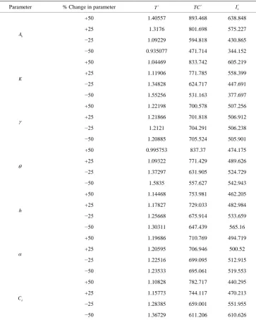
5. Sensitivity Analysis
We now study the effect of changes in the values of the system parameters A0, K, γ, θ, h, α and Cd on
the optimal cost and number of reorder. The sensitivity analysis is performed by changing each of the parameters by 50%, 25%, 25%− and −50% taking one parameter at a time and keeping the remaining parameters un- changed.
The analysis is based on the Example -1 and the results are shown in the Table 1. The following points are observed.
1) T*, TC* & I0* increase with increase in value of the parameter A0. Here *
,
T TC* & I0* are mod-
erately sensitive to change in A0.
2) T* decreases while TC* & I0* increase with increase in value of the parameter K. Here
* ,
T TC* &
* 0
I are moderately sensitive to change in K. 3) T* & I0* increase while
*
TC decreases with increase in value of the parameter γ. Here T*, TC* & I0*
are lowly sensitive to change in γ. 4) T* & I0* decrease while
*
Table 1. Sensitivity analysis.
Parameter % Change in parameter *
T *
TC *
0 I
0 A
+50 1.40557 893.468 638.848
+25 1.3176 801.698 575.227
−25 1.09229 594.818 430.865
−50 0.935077 471.714 344.152
K
+50 1.04469 833.742 605.219
+25 1.11906 771.785 558.399
−25 1.34828 624.717 447.691
−50 1.55256 531.163 377.697
γ
+50 1.22198 700.578 507.256
+25 1.21866 701.818 506.912
−25 1.2121 704.291 506.238
−50 1.20885 705.524 505.901
θ
+50 0.995753 837.37 474.175
+25 1.09322 771.429 489.626
−25 1.37297 631.905 524.729
−50 1.5835 557.627 542.943
h
+50 1.14468 753.981 462.205
+25 1.17827 729.033 482.984
−25 1.25668 675.914 533.659
−50 1.30311 647.439 565.16
α
+50 1.19686 710.769 494.719
+25 1.20595 706.946 500.52
−25 1.22516 699.095 512.915
−50 1.23533 695.061 519.553
d
C
+50 1.10828 782.717 440.295
+25 1.15773 744.117 470.213
−25 1.28385 659.001 551.955
−50 1.36729 611.206 610.626
are highly sensitive to change in θ. 5) T*
& * 0
I decrease while TC* increases with increase in value of the parameter h. Here T*, TC* & * 0 I
are moderately sensitive to change in h. 6) T*
& * 0
I decrease while TC* increases with increase in value of the parameter α. Here T*, TC* &
* 0
I are lowly sensitive to change in α. 7) T*
& * 0
I decrease while TC* increases with increase in value of the parameter Cd. Here
* ,
T TC* &
* 0
I are moderately sensitive to change in Cd.
6. Conclusions
allowed. This model is solved analytically by minimizing the total inventory cost. Finally, the proposed model has been verified by the numerical example along with sensitivity analysis.
In the future study, it is hoped to further extend the proposal model into several situations such as shortages being allowed and the consideration of multi-item problem. The suggested model can be extended for items having linear increasing demand, stock dependent demand, price dependent demand or power demand. This model can be extended to a three-parameter Weibull distribution or Gamma distribution deterioration. Further- more, it may also take partial backlogging into account when determining the optimal replenishment policy.
Acknowledgements
The authors would like to thank the editor and anonymous reviewers for their valuable and constructive com- ments, which have led to a significant improvement in the manuscript
REFERENCES
[1] F. Raafat, “Survey of Literature on Continuously Deteriorating Inventory Model,” Journal of the Operational Research Society, Vol. 42, No. 1, 1991, pp. 27-37.
[2] H. M. Wee, “Economic Production Lot Size Model for Deteriorating Items with Partial Back Ordering,” Computers and Indus- trial Engineering, Vol. 24, No. 3, 1993, pp. 449-458.
[3] N. H. Shah and Y. K. Shah, “Literature Survey on Inventory Model For Deteriorating Items,” Economics Annals, Vol. 44, 2000, pp. 221-237.
[4] S. K. Goyal and B. C. Giri, “Recent Trends in Modeling of Deteriorating Inventory,” European Journal of Operational Re- search, Vol. 134, No.1, 2001, pp. 1-16.
[5] R. Li, H. Lan and J. R. Mawhinney, “A Review on Deteriorating Inventory Study,” Journal of Service Science and Manage-
ment, Vol. 3, No. 1, 2010, pp.117-129.
[6] F. W. Harris, “Operations and Cost,” A. W. Shaw Company, Chicago, 1915, pp. 48-54.
[7] R. H. Wilson, “A Scientific Routine for Stock Control,” Harvard Business Review, Vol. 13, No. 1, 1934, pp. 116-128. [8] T. M. Whitin, “Theory of Inventory Management,” Princeton University Press, Princeton, 1957, pp. 62-72.
[9] P. M. Ghare and G. F. Schrader, “A Model for an Exponentially Decaying Inventory,” Journal of Industrial Engineering, Vol. 14, 1963, pp. 238-243.
[10] U. Dave and L. K. Patel, “(T, Si) Policy Inventory Model for Deteriorating Items with Time Proportional Demand,” Journal of the Operational Research Society, Vol. 32, 1981, pp. 137-142.
[11] K. J. Chung and P. S. Ting, “A Heuristic for Replenishment for Deteriorating Items with a Linear Trend in Demand,” Journal of the Operational Research Society, Vol. 44, 1993, pp. 1235-1241.
[12] H. M. Wee, “A dEterministic Lot-Size Inventory Model for Deteriorating Items with Shortages and a Declining Market,”
Computers and Operations Research, Vol. 22, No. 3, 1995, pp. 345-356 [13] V. K. Mishra, L. S. Singh and R. Kumar, “An Inventory Model for Deteriorating Items with Time-Dependent Demand and
Time-Varying Holding Cost under Partial Backlogging,” Journal of Industrial Engineering International, Vol. 9, No. 4, pp.
2013, pp. 1-5.
[14] H. J. Chang and C. Y. Dye, “An EOQ Model for Deteriorating Items with Time Varying Demand and Partial Backlogging,”
Journal of the Operational Research Society, Vol. 50, 1999, pp. 1176-1182.
[15] W. Ouyang and X. Cheng, “An Inventory Model for Deteriorating Items with Exponential Declining Demand and Partial Backlogging,” Yugoslav Journal of Operation Research, Vol. 15, No. 2, 2005, pp. 277-288.
[16] P. L. Abad, “Optimal Pricing and Lot-Sizing under Conditions of Perishability and Partial Backordering,” Management Science,
Vol. 42, No. 8, 1996, pp. 1093-1
[17] P. L. Abad, “Optimal Price and Order-Size for a Reseller under Partial Are Backlogging,” Computers and Operations Research,
Vol. 28, No. 1, 2001, pp. 53-65
[18] N. H. Shah and N. Raykundaliya, “Retailer’s Pricing and Ordering Strategy for Weibull Distribution Deterioration under Trade Credit in Declining Market,” Applied Mathematical Sciences, Vol. 4, No. 21, 2010, pp. 1011-1020.
[19] T. Singh and H. Pattnayak, “An EOQ Model for Deteriorating Items with Linear Demand, Variable Deterioration and Partial Backlogging,” Journal of Service Science and Management, Vol. 6, No. 2, 2013, pp. 186-190.
[20] C. K. Tripathy and U. Mishra, “Ordering Policy for Weibull Deteriorating Items for Quadratic Demand with permissible Delay in Payments,” Applied Mathematical Science, Vo. 4, No. 44, 2010, pp. 2181-2191.
[21] T. Singh and H. Pattnayak, “An EOQ Model for A Deteriorating Item with Time Dependent Exponentially Declining Demand under Permissible Delay in Payment,” IOSR Journal of Mathematics, Vol. 2. No. 2, 2012, pp. 30-37.
[22] T. Singh and H. Pattnayak, “An EOQ Model for a Deteriorating Item with Time Dependent Quadratic Demand and Variable Deterioration under Permissible Delay in Payment,” Applied Mathematical Sciences, Vol. 7, No. 59, 2013, pp. 2939-2951. [23] R. Amutha and E. Chandrasekaran, “An EOQ Model for Deteriorating Items with Quadratic Demand and Time Dependent
Holding Cost,” International Journal of Emerging Science and Engineering, Vol. 1, No. 5, 2013, pp. 5-6.
Notations
The following notations have been used in developing the model. 1) A0: the fixed ordering cost per order..
2) I t
( )
: the inventory at time t, 0≤ ≤t T .3) D t
( )
: the exponential demand rate where D t( )
=Ke−γt, K>0, γ >0, Kγ , are constants, K de-notes constant demand rate and γ denotes the rate of change of demand rate.4) θ
( )
t : the constant deterioration rate of an item where θ( )
t =θ(
0< <θ 1)
and 0< <γ θ. 5) h t( )
: the time-varying holding cost per unit time where h t( )
= +h αt, h>0 and α >0. 6) Cd: the cost of each deteriorated unit.7) T: the length of the ordering cycle. 8) I0: the economic order quantity. 9) TC: the total cost per unit time. 10) T*: the optimal length of the cycle. 11) I0
∗