Measuring the value of life: exploring a
new method for deriving the monetary
value of a QALY
Tilling, C and Krol, M and Tsuchiya, A and Brazier, J and
van Exel, J and Brouwer, W
The University of Sheffield
2009
Online at
https://mpra.ub.uni-muenchen.de/29911/
HEDS Discussion Paper 09/14
Disclaimer:
This is a Discussion Paper produced and published by the Health Economics and Decision Science (HEDS) Section at the School of Health and Related Research (ScHARR), University of Sheffield. HEDS Discussion Papers are intended to provide information and encourage discussion on a topic in advance of formal publication. They represent only the views of the authors, and do not necessarily reflect the views or approval of the sponsors.
White Rose Repository URL for this paper: http://eprints.whiterose.ac.uk/10879/
Once a version of Discussion Paper content is published in a peer-reviewed journal, this typically supersedes the Discussion Paper and readers are invited to cite the published version in preference to the original version.
Published paper
None.
Measuring the value of life: Exploring a new method for
deriving the monetary value of a QALY
Carl Tilling*
1, Marieke Krol
2, Aki Tsuchiya
1,3, John Brazier
1,
Job van Exel
2, Werner Brouwer
2* Corresponding author: [email protected]
1. School of Health and Related Research, University of Sheffield
2. Institute for Medical Technology Assessment, Erasmus University, Rotterdam
3. Department of Economics, University of Sheffield
Introduction
Economic evaluations of new health technologies now typically produce an incremental cost per Quality Adjusted Life Year (QALY) value. The QALY is a measure of health benefit that combines length of life with quality of life, where quality of life is assessed on a scale where zero represents a health state equivalent to being dead and one represents full health (Weinstein and Stason, 1977). The challenge for decision makers, such as the Treasury, is to determine the appropriate size of the healthcare budget. Bodies, such as the National Institute for Health and Clinical Excellent (NICE) in the U.K., must then determine how much it can afford to pay for a gain of one QALY, while operating under this fixed budget. While there is no fixed cost-effectiveness threshold and each intervention is assessed on a case by case basis (Rawlins and Culyer, 2004), under normal circumstances the threshold will not be below £20,000 and not above £30,000 per QALY (NICE, 2008).
Gyrd-Hansen 2003). However, WTP has a number of known problems, most notably its insensitivity to scope (Olsen et al. 2004). In this paper we present an alternative approach to estimating the monetary value of a QALY (MVQ), which is based upon a Time Trade Off (TTO) exercise of income with health held constant at perfect health. We present the methods and theory underlying this experimental approach and some results from an online feasibility study in the Netherlands.
Background
Willingness to Pay (WTP) has been used to estimate the MVQ in two ways. The first has been to elicit the WTP for a reduction in the risk of death and then calculate the value of a statistical life, from which the MVQ can be inferred. Early studies using this approach produced WTP per QALY estimates ranging from £51,000 to £101,000 (in 2003 prices) (e.g. Johannesson and Meltzer 1998, Hirth et al. 2000, Abelson 2003). More recently Mason et al. (2009) have used this method and produced estimates ranging from £24,219 to £70,896. The second approach has been to directly elicit a WTP value for changes in health status. This can be through hypothetical generic quality of life improvements (Gyrd-Hansen 2003; Prades et al. 2009), hypothetical increases in life expectancy (Johannesson and Johansson 1997; Johnson et al. 1998), improvements in own health amongst a patient population (King et al. 2005) or alleviation of a specific health condition (Lundberg 1999). Estimates from the direct approach are generally much lower than from the value of a statistical life approach. However, the most recent study, by Prades et al. (2009), produced estimates ranging from €4,585 to €123,724.
decisions in health care contingent valuation studies. However, even if the WTP study is designed appropriately a number of other problems have been shown to be inherent in the WTP method. These include insensitivity to scope (Olsen et al. 2004), strategic behaviour (Hackl and Pruckner, 2005), the restriction of personal income (O’Brien and Drummond, 1994) and protest responses (Dalmau-Matarrodona, 2001).
Insensitivity to scope arises if respondents’ WTP does not change in response to the size of the outcome being valued. Evidence of insensitivity to scope concerns economists because it contradicts the fundamental principles of neo-classical theory: since ‘more is better’ consumers should be prepared to sacrifice more money to achieve it (albeit at a diminishing rate). From a practical perspective, if WTP results are to be used to inform the cost-effectiveness threshold applied in health care allocation decisions it is crucial that two health gains of different sizes receive different values. Olsen et al. (2004) asked respondents their WTP for either 100 or 50 patients, cancer radiotherapy for either 300 or 150 patients or a helicopter ambulance that would save either 10 or 15 lives. The results showed no significant differences in WTP for different sized health effects. Chestnut et al. (1996) found that meanWTP to avoid four angina attacks did not differ significantly from mean WTP to avoid eight attacks. A number of studies dealing with different sizes of risk reductions have also found evidence in support of scope insensitivity (see Smith and Desvouges 1987; Jones-Lee, Loomes and Phillips 1995). However, Kartman et al. (1996a,b) and O’Conor et al. (1998) all found evidence against insensitivity to scope making it hard to draw definite conclusions.
(see Donaldson 1999), but this still requires the assumption that individuals in the same income category have the same marginal utility of income.
Strategic behaviour (free-riding) may occur in WTP studies in two directions. Firstly, if respondents think they will actually have to pay the amount they reveal they may underbid. Alternatively, if respondents do not believe they will actually have to pay their stated WTP amount, but they want to influence the provision of the good in question, we might expect them to overbid. In the environmental field Bohm (1984), Brubaker (1984) and Milon (1989) all found only minor strategic effects. There is limited available evidence in the health care field. Hackl and Pruckner (2005) test for free riding by asking Austrian respondents their WTP for the provision of health-related Red Cross services. They found only a few cases that would point towards free-riding behaviour.
According to Dalmau-Matarrodona (2001) non-responses in WTP exercises fall into four categories: don’t know, real zeros, protest zeros and outliers. He defines protest zeros as those coming from respondents who have negative attitudes towards the good in question and hence give a zero response, when their real value is positive. The standard approach is to discard these observations. However, this may cause problems through information loss and reduced sample size, and the results may be biased if the characteristics of those respondents giving protest responses differ from the rest of the sample. Innovative methods to include protest responses have been experimented with (Dalmau-Matarrodona 2001 uses a double hurdle modelling approach) but protest responses remain a problem in WTP studies.
receive from the good or service paid for. However, under a publicly funded health scheme, the payment is largely unrelated to the benefits that the payee will obtain. The relevant WTP question becomes how much the individual is prepared to pay for another’s health, with the caveat that they too can potentially benefit from the services that others receive. Therefore, it is entirely possible for an individual’s personal WTP to diverge from their fair share of social WTP.
Attempting to derive an MVQ has been termed as ‘building a bridge between CBA and CEA’ (Dolan and Edlin, 2002). This is because if an MVQ is identified, then the costs of a treatment can be directly compared with the benefits, expressed in monetary net benefit terms and interpreted in standard welfare economic terms. However, Dolan and Edlin (2002) have shown that some rather restrictive and unrealistic assumptions have to be made to build this bridge. The approach of Johannesson and Meltzer (1998) requires that incomes be held constant across individuals for WTP to be proportional to the QALY gain. Dolan and Edlin relax this assumption and show that health must be additively separable to consumption in the utility function, since the relationship between health and income would influence the ability of an individual to enjoy consumption. Another attempt to link CBA and CEA, by Bleichrodt and Quiggin (1999), differs in that individual WTP figures are used, but this leads to differences in thresholds across individuals. Ultimately, Dolan and Edlin argue that it is not possible to link CBA and CEA if: (i) the axioms of EU theory hold; (ii) the QALY model is valid in a welfare economic sense; and (iii) illness hinders the ability to enjoy consumption.
Methods
Data were gathered as part of a study seeking to determine whether respondents in TTO exercises consider the effects the states might have upon their income. Data were gathered through an online self-complete questionnaire administered in the Netherlands. Invitations were sent out to a subset of an existing panel of potential survey respondents in order to obtain a representative sample of 300 members of the Dutch general public. We selected respondents between the ages of 18 and 65 as we felt that questions about income were most relevant for people in this age bracket. The data collection was performed by an online market research company (Survey Sampling International; www.surveysampling.com). Following a number of background, ranking and Visual Analogue Scale (VAS) questions respondents were presented with five different TTO exercises (see Tilling et al. 2009 for more details).
Two of these TTO exercises were relevant for this study and all respondents answered both:
TTO 1: Trading years to avoid an income loss in perfect health (equivalent
loss)
“You can live for 10 years in perfect health with (100 - Y)% of your current annual income for each year and then die or you can live for a shorter period of time in perfect health with your current annual income for each year and then die.”
TTO 2: Trading years to achieve an income gain in perfect health
(compensating gain)
Three income change levels (Y) were used: 20%, 40% and 60%, and respondents were randomised to one of these three income change levels which they then received in both TTO1 and TTO2. Since the survey was administered in an online self-complete fashion there was no iterative process. Respondents were simply asked to state how many years with higher income, was equivalent to 10 years with lower income. It should also be noted that all respondents received the two questions in the same order: TTO1 followed by TTO2. Therefore, we cannot rule out the possibility that responses to TTO2 are affected by respondent’s having already seen TTO1.
Essentially both questions can be interpreted as WTP questions. However, while standard WTP questions ask people to trade money for an improvement in survival prospects, and thus by implication, length of life or health, these questions ask people to trade length of life for an improvement in income. Respondents are paying in years of life. TTO 1 is a form of equivalent variation. Equivalent variation is ‘the amount of money a consumer would pay to avert a price increase’ (Hicks 1939). In TTO1 the consumer is faced with a fall in income of X%, which is essentially the same as an increase in prices. They are then asked how many years of life (rather than how much money) they would pay to avoid this ‘price increase’. Similarly, TTO2 can be considered a form of compensating variation. Compensating variation is ‘the amount of additional money a consumer requires to reach his initial level of utility after a change in prices’ (Hicks 1939). For a drop in prices, the amount of additional money compensation will be negative. TTO2 essentially corresponds to a compensating variation that identifies the number of years payable that would let the individual maintain the initial level of utility after a drop in prices, or increase in income.
€80,000. Therefore, using prospective lifetime income values and an additive utility function, this point of indifference gives us the following information:
10U (Perfect Health) + €800,000 = 9U (Perfect Health) + €900,000 (1) 10U (Perfect Health) – 9U (Perfect health) = €900,000 - €800,000 (2) U (Perfect Health) = €100,000 (3)
This method requires that we assume additivity between health and income in the utility function. In reality it is likely that the utility from a year in perfect health will be higher when combined with a higher amount of income. Therefore, we make the same assumption as Johannesson and Meltzer (1998), and hence do not avoid Dolan and Edlin’s (2002) impossibility theorem. We also assume a constant marginal rate of substitution between health and income. Relaxing this assumption would require us to estimate an indifference curve across a range of values. Unfortunately we do not have enough data points for this to be possible in this study.
The compensating gain data from TTO2 is analysed in a similar fashion to the equivalent loss data in TTO1. Consider a respondent who is indifferent between 10 years with their current income and 9 years with 120% of their current income. Their income is, once again, €100,000 per year:
10 U(PH) + €1000,000 = 9 U(PH) + €1080,000 (4) 10U (PH) – 9U (PH) = €1080,000 – €1000,000 (5)
U(PH) = €80,000 (6)
Notice that a compensating gain of €20,000 has led to a lower MVQ estimate than a gain of €20,000 in the equivalent loss question. This is because, as a proportion, €20,000 is larger in the equivalent loss question.
each question the compensating gain question will give lower results. However, based on the assumption of diminishing marginal utility of income we would expect the compensating gain results to give a higher MVQ than the equivalent loss. Respondents will trade fewer years in order to achieve an increase in income, hence each year is valued more highly in monetary terms. This is also supported by the findings of Kahneman and Tversky (1979): through a series of probabilistic choices they found risk aversion in choices involving sure gains, and risk seeking involving sure losses. This suggests that respondents will trade more years in the equivalent loss questions than in the compensating gain questions, which would lead to higher MVQ values in the latter.
Respondent Income
In order to determine the level of “current annual income” for each respondent, respondents were asked to choose the income bracket within which their monthly income fell in the background characteristics questions. For our analysis these income brackets were converted into numerical values using the mid-point of each bracket (Layard et al. 2008). For respondents in the lowest income bracket an income of two thirds of the upper limit of the bracket was used. For respondents in the highest income bracket an income of 1.5 of the lower income limit of the bracket was assumed (Layard et al. 2008).
Non-Traders
each individual and then aggregate (as outlined above), then these non-traders cause a problem because the left hand side of equation (2) becomes 0, meaning that the equation would give an indeterminate value. There are two possible responses to this problem: the first (the “individual approach”) is to exclude all respondents that did not trade, and the second (the “aggregate approach”) is to aggregate at the start of the calculations i.e. use aggregate income and aggregate number of years traded. We present results from both approaches.
Negative Values
One further problem is the generation of negative MVQ values. For TTO1 if the percentage of life years the respondent is prepared to give up is larger than the percentage income loss he is faced with then his MVQ will be negative. In other words if the respondent is faced with 20% income loss, and if they trade more than 2 years of life their MVQ value will be negative. If they trade exactly 2 years their MVQ value will be zero. So for the 40% loss they can not trade more than 4 years, and for the 60% loss they cannot trade more than 6 years. For TTO2 the relationship is not linear. For 20% gain they cannot trade more than 1.666 years, for 40% gain they can not trade more than 2.86 years and for 60% gain they can not trade more than 3.75 years. In the individual approach we truncate negative MVQ values at 0. In the aggregate approach we leave the number of years traded unchanged.
Results
standard TTO question of hypothetical health states. Extreme non-traders were in better health than traders, though this was only significant at the 10% level.
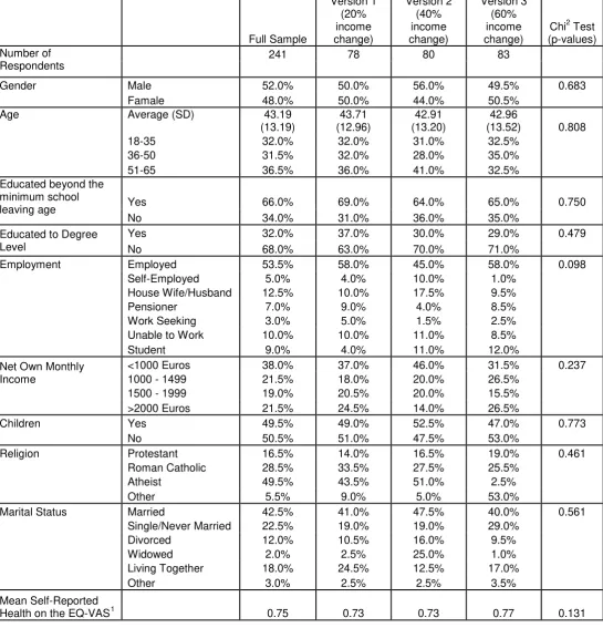
Table 1 – Background characteristics by income change level Full Sample Version 1 (20% income change) Version 2 (40% income change) Version 3 (60% income change)
Chi2 Test (p-values) Number of
Respondents
241 78 80 83
Gender Male 52.0% 50.0% 56.0% 49.5% 0.683
Famale 48.0% 50.0% 44.0% 50.5%
Age Average (SD) 43.19
(13.19) 43.71 (12.96) 42.91 (13.20) 42.96
(13.52) 0.808
18-35 32.0% 32.0% 31.0% 32.5%
36-50 31.5% 32.0% 28.0% 35.0%
51-65 36.5% 36.0% 41.0% 32.5%
Educated beyond the minimum school
leaving age Yes 66.0% 69.0% 64.0% 65.0% 0.750
No 34.0% 31.0% 36.0% 35.0%
Educated to Degree Level
Yes 32.0% 37.0% 30.0% 29.0% 0.479
No 68.0% 63.0% 70.0% 71.0%
Employment Employed 53.5% 58.0% 45.0% 58.0% 0.098
Self-Employed 5.0% 4.0% 10.0% 1.0%
House Wife/Husband 12.5% 10.0% 17.5% 9.5%
Pensioner 7.0% 9.0% 4.0% 8.5%
Work Seeking 3.0% 5.0% 1.5% 2.5%
Unable to Work 10.0% 10.0% 11.0% 8.5%
Student 9.0% 4.0% 11.0% 12.0%
Net Own Monthly Income
<1000 Euros 38.0% 37.0% 46.0% 31.5% 0.237
1000 - 1499 21.5% 18.0% 20.0% 26.5%
1500 - 1999 19.0% 20.5% 20.0% 15.5%
>2000 Euros 21.5% 24.5% 14.0% 26.5%
Children Yes 49.5% 49.0% 52.5% 47.0% 0.773
No 50.5% 51.0% 47.5% 53.0%
Religion Protestant 16.5% 14.0% 16.5% 19.0% 0.461
Roman Catholic 28.5% 33.5% 27.5% 25.5%
Atheist 49.5% 43.5% 51.0% 2.5%
Other 5.5% 9.0% 5.0% 53.0%
Marital Status Married 42.5% 41.0% 47.5% 40.0% 0.561
Single/Never Married 22.5% 19.0% 19.0% 29.0%
Divorced 12.0% 10.5% 16.0% 9.5%
Widowed 2.0% 2.5% 25.0% 1.0%
Living Together 18.0% 24.5% 12.5% 17.0%
Other 3.0% 2.5% 2.5% 3.5%
Mean Self-Reported
Health on the EQ-VAS1 0.75 0.73 0.73 0.77 0.131
1
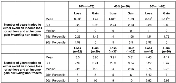
Table 2 – Number of years traded both including and excluding non-traders
20% (n=78) 40% (n=80) 60% (n=83)
Loss Gain Loss Gain Loss Gain
Number of years traded to either avoid an income loss
or achieve and an income gain including non-traders
Mean 0.992 1.47 1.812** 1.33 2.451 1.511***
SD 2.23 2.96 2.74 2.63 3.28 2.89
Median 0 0 0 0 1 0
75th Percentile 0.25 1.42 4 1.08 4.5 1.75
90th Percentile 4.92 5 5 5.5 8.92 5
Loss (n=22)
Gain (n=29)
Loss (n=37)
Gain (n=28)
Loss (n=46)
Gain (n=30)
Number of years traded to either avoid an income loss
or achieve and an income gain excluding non-traders
Mean 3.5 3.95 3.91 3.81 4.43 4.17
SD 2.99 3.74 2.83 3.24 3.27 3.47
Median 2.25 2.5 4 2.96 3.75 2.75
75th Percentile 5 5 5 6 6.42 7
90th Percentile 9 10 9 10 9.92 9.96
Table 2 shows the mean number of years respondents were willing to trade, in both the compensating gain and equivalent loss questions, with and without respondents who did not trade any time. Looking at the values for the larger sample, for two of the income change levels respondents are prepared to trade more years to avoid an income loss than they are to achieve an income gain. However, these differences are only significant for the 60% income
change level (tested through t-test and signalled by 1***, the number indicating the points of comparison and the *’s indicating the level of significance: * 10%, **5%, ***1%). The median values are 0 in all but one case, which is a product of the large numbers of non-traders. Mann-Whitney rank-sum tests were performed comparing the values for the different income levels, both for equivalent loss and compensating gain values. Comparison between 20% and 40% equivalent loss proved significant at the 10% level, while comparison between 20% and 60% equivalent loss proved significant at the 1% level. For the equivalent loss questions the standard deviations generally increase as the level of loss increases, while no clear relationship can be observed for the gain questions. The 75th and 90th percentiles show the skewness caused by the non-traders.
For the smaller sample, without non-traders, the mean number of years traded is considerably higher across all questions. More years are traded in the equivalent loss questions for the two more severe income change levels, but these differences are not significant. None of the t-tests comparing values across the different income levels for both losses and gains are significant.
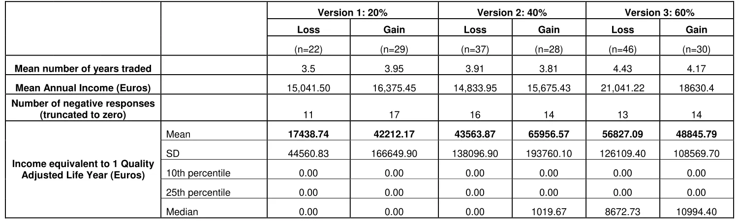
Table 3 – MVQ values calculated at the individual level (excluding non-traders)
Version 1: 20% Version 2: 40% Version 3: 60%
Loss Gain Loss Gain Loss Gain
(n=22) (n=29) (n=37) (n=28) (n=46) (n=30)
Mean number of years traded 3.5 3.95 3.91 3.81 4.43 4.17
Mean Annual Income (Euros) 15,041.50 16,375.45 14,833.95 15,675.43 21,041.22 18630.4
Number of negative responses
(truncated to zero) 11 17 16 14 13 14
Income equivalent to 1 Quality Adjusted Life Year (Euros)
Mean 17438.74 42212.17 43563.87 65956.57 56827.09 48845.79
SD 44560.83 166649.90 138096.90 193760.10 126109.40 108569.70
10th percentile 0.00 0.00 0.00 0.00 0.00 0.00
25th percentile 0.00 0.00 0.00 0.00 0.00 0.00
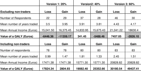
Table 4 – MVQ values calculated at the aggregate level with and without non-traders
Version 1: 20% Version2: 40% Version 3: 60%
Excluding non-traders Loss Gain Loss Gain Loss Gain
Number of Respondents 22 29 37 28 46 30
Mean number of years traded 3.5 3.95 3.91 3.81 4.43 4.17
Mean Annual Income (Euros) 15,041.50 16,375.45 14,833.95 15,675.43 21,041.22 18630.4
Value of a QALY (Euros) -6446.36 -11359.17 341.45 -5488.46 7457.05 -2826.10
Including non-traders Loss Gain Loss Gain Loss Gain
Number of respondents 78 78 80 80 83 83
Mean number of years traded 0.99 1.47 1.81 1.33 2.45 1.51
Mean Annual Income (Euros) 17471.38 17471.38 15771.30 15771.30 20828.82 20828.82
Value of a QALY (Euros) 17824.34 2804.93 19082.40 25352.66 30180.54 49437.41
Table 4 shows the MVQ values calculated using aggregate values, first without the non-traders and then with the non-traders. In all but two cases using the aggregate approach without the non-traders produces negative MVQ values. In the two cases where positive values are produced comparison with the results from the individual approach shows that the aggregate approach produces much lower estimates. Considering the results from the aggregate approach, with non-traders, the estimates range from €2,804.93 to €49,437.41. These values are closer to those generated through the individual approach, especially for 20% loss and 60% gain which produce values very similar to the individual approach.
Table 5 – Weighted mean QALY values for different income brackets for both the individual approach and the aggregate approach
` Version1: 20% Version 2: 40% Version 3: 60%
Income Level Loss n Gain n Loss n Gain n Loss n Gain n
Weighted Mean QALY value
Individual Approach
Less than 12,000 euros 22,522.93 11 19,941.96 14 13,235.43 18 48,448.81 11 117,113.60 13 68,606.70 11 45,836.73
12,000 to 17,999 euros 22,800.02 5 11,294.11 4 104,285.80 7 36,571.42 7 17,863.63 11 35,999.99 4 39,096.76
18,000 to 23,999 euros 0.00 2 0.00 5 82,579.01 7 149,400.10 7 56,405.78 9 36,120.00 5 66,060.17
>24,000 euros 5,475.00 4 149,964.90 6 13,114.29 5 4,015.39 3 29,801.30 13 38,609.99 10 43,239.61
22 29 37 28 46 30
Aggregate Approach
Less than 12,000 euros 5576.76 29 0.00 29 7421.69 37 16976.84 37 19661.98 26 13007.31 26 10,401.49
12,000 to 17,999 euros 15000.00 14 24372.88 14 23535.65 16 28220.67 16 22190.08 22 112570.56 22 41,769.77
18,000 to 23,999 euros 40046.51 16 0.00 16 40810.15 16 16932.05 16 22674.18 13 71487.57 13 30,985.80
>24,000 euros 34747.61 19 8999.70 19 33449.06 11 40953.74 11 29389.61 22 38094.48 22 30,137.31
Discussion and Conclusion
The aim of this study was not to present a definitive MVQ for the Netherlands, but to test the feasibility of an alternative method of eliciting an MVQ. The results from this small-scale online study suggest that the compensating gain and equivalent loss TTO exercises have potential, but a number of problems must be overcome before it can challenge WTP as the dominant method of estimating an MVQ. Generally respondents in our new method give up more years when faced with a larger income change level, thus suggesting some sensitivity to scope. However, these differences are not always significant and are never significant without the ‘non traders’. Studies with larger sample sizes may be able to determine whether the method is sensitive to scope.
approach is to be tested further, it would be most appropriate to use an interview method of elicitation. However, we cannot rule out the possibility that these responses are either meaningful responses or protest responses. If they are meaningful responses they would highlight a problem with the method – those who do not trade any time cannot be included in the analysis. If they are protest responses they would suggest our method is unlikely to overcome this particular weakness of WTP.
A serious problem with the TTO based approach is the elicitation of negative MVQ values. Referring to Equation 7, given the assumption of additivity, a rational respondent should not trade more than two years (i.e. a value of eight on the right hand side of the equation) because to do so would mean a lower total lifetime income. However, in reality it is plausible that individuals may wish to live for a shorter period of time with high income than for a longer period of time with lower income, even though their total lifetime income may be lower. It is also likely that respondents may not have been able to determine the point at which their lifetime income became lower. If these questions were tested through an interview elicitation procedure it may be possible to use a visual aid that would attempt to make it clearer to respondents the point at which lifetime income in the trading scenario becomes lower than lifetime income in the alternative scenario. This could be done by adapting the standard MVH TTO board to include an additional strip for lifetime income. This may reduce the number of respondents trading too many years.
this approach would entail further dependence upon the assumption of no interactions between health and income. This assumption, one of the impossibility theorem criteria set out by Dolan and Edlin (2002) is not avoided in this study. The MVQ value elicited is essentially determined by the choice of income change level. A large scale study would make it possible to gain values for enough income change levels to estimate an indifference curve between health and income. An average MVQ value across a range of income change levels could then be estimated.
It is not clear whether the ‘individual’ approach or the ‘aggregate’ approach is preferable. The use of the aggregate approach without non-traders does not appear to be a credible option due to the generation of negative values. However, the validity of results using the aggregate approach with non-traders is questionable as these valuations may be meaningless strategic non-trades. On the other hand, the individual approach has the drawback of small sample sizes. Before a preference can be formed more research using face to face interviews is needed to try and determine whether the non-trades are strategic or true indicators of preference, and hence whether the calculation method needs to be able to accommodate them. Regardless of which method is used if the results are to be generalised to infer an MVQ it is crucial that the income of the sample is representative of society. Even if this method can be refined to estimate a reliable MVQ this does not overcome the problems of inferring a social value of a QALY from this information.
Acknowledgements
We would like to thank Jan van Busschbach who discussed a version of this paper at the Dutch HESG in May 2009, and Paul McNamee who discussed the same version of the paper at Sheffield HESG in July 2009. We would also like to thank Phil Shackley, who refereed this paper for inclusion in the ScHARR DP series, and Richard Edlin who provided helpful feedback and comments. Finally, we would like to thank the respondents who took part in this study. Carl Tilling is an ESRC funded PhD student.
References
Abelson, P. 2003. The value of life and health for public policy. The Economic Record, 79: S2-S13
Bleichrodt, H., Quiggin, J. 1999. Life-cycle preferences over consumption and health: when is cost-effectiveness analysis equivalent to cost-benefit analysis? Journal of Health Economics, 18 (6): 681-708
Bohm, P. 1984. Revealing demand for an actual public good. Journal of Public Economics, 24: 135-151
Brubaker, E.R. 1984. Demand disclosures and conditions on exclusion: An experiment. The Economic Journal, 94: 536-553.
Chestnut, K.L., Lambert, W., Rowe, R. 1996. Measuring heart patient’ willingness to pay for changes in angina symptoms. Medical Decision Making,
16(1): 65-77
Dalmau-Matarrodona, E. 2001. Alternative approaches to obtain optimal bid values in contingent valuation studies and to model protest zeros. Health Economics, 10: 101-118.
Dolan, P., Edlin, R. 2002. Is it really possible to build a bridge between cost-benefit analysis and cost-effectiveness analysis? Journal of Health Economics,
21: 827-843
Donaldson, C. 1999. Valuing the benefits of publicly-provided health care: does ‘ability to pay’ preclude the use of ‘willingness to pay’? Social Science and Medicine, 49: 551-563
Frew, E.J. 2003. Willingness to pay for colorectal cancer screening: a comparison of elicitation formats. PhD Thesis. University of Nottingham.
Gold MR, Siegel JE, Russell LB, Weinstein MC. Cost-Effectiveness in Health and Medicine. Oxford: Oxford University Press, 1996.
Gyrd-Hansen, D. 2003. Willingness to pay for a QALY. Health Economics, 112:
Hackl, F., Pruckner, G.J. 2005. Warm glow, free-riding and vehicle neutrality in a health-related contingent valuation study. Health Economics, 14 (3): 293-306.
Hayes, K., Lockwood, M., Anderson, G. 1992. Estimating the Benefits of Water Quality Improvements in the Upper Narragansett Bay. Marine Resource Economics, 7: 75-85
Hicks, J.R. 1939. Value and capital: An enquiry into some fundamental principles of economic theory. Oxford: Clarendon Press.
Hirth, R.A., Chernew, M.E., Miller, E., Fendrick, M., Weisser, W.G. 2000. Willingness to pay for a quality adjusted life year: in search of a standard. Medical Decision Making, 20: 332-342.
Johannesson, M., Johansson, P-O. 1997. Quality of life and the WTP for an increase in life expectancy at an advanced age. Journal of Public Economics,
65: 219-228
Johannesson, M., Meltzer, D. 1998. Some reflections on cost-effectiveness analysis. Health Economics, 7 (1): 1-7
Johnson, F.R., Desvousges, W.H., Ruby, M., Stieb, D. and De Civita, P. 1998. Eliciting stated health preferences: an application to willingness to pay for longevity. Medical Decision Making, 18: S57-S67.
Jones-Lee, M.W., Loomes, G., Phillips, P.R. 1995. Valuing the prevention of non-fatal road injuries: Contingent valuation vs standard gambles. Oxford Economic Papers, 47: 676-695
Kahneman, D., Tversky, A. 1979. Prospect Theory: An Analysis of Decision under Risk. Econometrica, 47(2): 263-291
Kartmann, B., Nils-Olov, S., Magnus, J. 1996a. Valuation of health changes with the contingent valuation method: a test of scope and question order effects. Health Economics, 5: 531-541.
Kartman, B., Andersson, F., Johannesson, M. 1996b. Willingness to pay for reduction in angina pectoris attacks. Medical Decision Making, 16: 248-253 King Jr., J.T., Tsevat, J., Lave, J.R., Roberts, M.S. 2005. Willingness to pay for a quality adjusted life year implications for societal health care resource allocation. Medical Decision Making, 25 (6): 667-677.
Layard, R., Mayraz, G., Nickell, S. 2008. The marginal utility of income. Journal of Public Economics, 92 (8): 1846 – 1857.
Lundberg, L., Johannesson, M., Silverdahl, M., Hermansson, C., Lindberg, M. 1999. Quality of life, health-state utilities and willingness to pay in patients with psoriasis and atopic eczema. British Journal of Dermatology, 141: 1067-75 Mason, H., Jones-Lee, M., Donaldson, C. 2009. Modelling the Monetary Value of a QALY: A New Approach based on UK data. Health Economics, 18: 933-950 Milon, W.J. 1989. Contingent Valuation experiments for strategic behavior. Journal of Environmental Economics and Management, 17: 293-308
National Institute for Clinical Excellence. NICE guide to the methods of technology appraisal. NICE, UK, 2008.
O’Brien, B.J., Gafni, A. 1996. When Do the “Dollars” Make Sense? Toward a conceptual framework for contingent valuation studies in health care. Medical Decision Making, 16: 288-299
Olsen, J.A., Donaldson, C., Pereira, J. 2004. The insensitivity of ‘willingness-to-pay’ to the size of the good: New evidence for health care. Journal of Economic Psychology, 25: 445-460
Prades, J.L.P, Loomes, G., Brey, R. 2009. Trying to estimate a Monetary Value for the QALY. Journal of Health Economics, 28: 553-562
Rawlins, M.D., Culyer, A.J. 2004. National Institute for Clinical Excellence and its value judgements. BMJ 329:224-227
Smith, R., Richardson, J. 2005. Can we estimate the ‘social’ value of a QALY? Four core issues to resolve. Health Policy, 74: 77-84
Smith, V.K., Desvouges, W.H., 1987. An empirical analysis of the economic value of risk changes. Journal of Political Economy, 95(1): 89-114
Stewart, J.M., O’Shea, E., Donaldson, C., Shackley, P. 2002. Do ordering effects matter in willingness-to-pay studies of health care? Journal of Health Economics, 21: 585-599.
Tilling, C., Krol, M., Tsuchiya, A., Brazier, J., Van Exel, J., Brouwer, W.B.F. 2009. The impact of losses in income due to ill health: Does the EQ-5D reflect lost earnings? Health Economics and Decision Science Discussion Paper Series, School of Health and Related Research, University of Sheffield.
Van Nooten FE, Koolman X, Brouwer WBF. Thirty Down, Ten to Go? Health Economics, in press.