Estimation of Area under Receiver Operating Characteristic Curve for Bi Pareto and Bi Two Parameter Exponential Models

http://dx.doi.org/10.4236/ojs.2014.41001

Estimation of Area under Receiver Operating

Characteristic Curve for Bi-Pareto and Bi-Two

Parameter Exponential Models

Bhavna Kaushal, Kanchan Jain, Suresh K. Sharma Department of Statistics, Panjab University, Chandigarh, India

Email: [email protected], [email protected], [email protected]

Received November 13, 2013; revised December 13, 2013; accepted December 20,2013

Copyright © 2014 Bhavna Kaushal et al. This is an open access article distributed under the Creative Commons Attribution License, which permits unrestricted use, distribution, and reproduction in any medium, provided the original work is properly cited. In accor- dance of the Creative Commons Attribution License all Copyrights © 2014 are reserved for SCIRP and the owner of the intellectual property Bhavna Kaushal et al. All Copyright © 2014 are guarded by law and by SCIRP as a guardian.

ABSTRACT

In this paper, we find the ROC curves for Bi-Pareto and Bi-two parameter exponential distributions. Theoretical, parametric and non-parametric values of area under receiver operating characteristic (AUROC) curve for dif- ferent parametric combinations have been calculated using simulations. These values are compared in terms of root mean square and mean absolute errors. The results are demonstrated for two real data sets.

KEYWORDS

ROC; AUROC; Pareto; Two Parameter Exponential; Root Mean Square Error; Mean Absolute Error

1. Introduction

Receiver operating characteristic (ROC) curves have become the standard tool for evaluating the discriminatory power of medical diagnostic tests and are commonly used in assessing the predictive ability of binary regression models. ROC curve is a diagnostic tool that helps in determining the accuracy of a test conducted on a person to know whether a particular disease is present or not. In a typical setting, one has a binary indicator and a set of predictors or marker values. The goal is to see how well the marker values predict the binary indicator. The principal idea is to dichotomize the marker at various thresholds and compute the resulting sensitivity and speci- ficity. Sensitivity of a test is defined as the probability of a positive test result when the disease is present and specificity is the probability of a negative test result when disease is absent. Sensitivity is also known as True Positive Rate (TPR) and specificity is known as False Negative Rate (FNR). False Positive Rate is termed as (1-specificity). ROC curve is obtained by plotting the sensitivity versus (1-specificity).

In credit rating models in finance, sensitivity is termed as “Hit Rate” (HR) whereas (1-specificity) is known as “False Alarm Rate” (FAR). If the rating score of the debtor is lower than a cut-off value C, he is treated a de- faulter. Otherwise, he is a non-defaulter.

Hence

( )

Total number of defaulters =

and

( )

Total number of non-defaulters =

( )

{

}

The area under ROC curve (AUROC) is a widely used summary index [3-6]. It is the average TPR taken uni- formly over all FPRs on (0, 1) and written as

( )

{

}

1 1

0

d

AUROC=

∫

For credit rating models,

[

]

(

)

1

0

d

AUROC=

∫

The area under ROC curve is

• 0.5 if the model does not have discriminative quality;

• between 0.5 and 1.0 for a reasonable model;

• if the model is perfect.

There are many methods, parametric as well as non-parametric, to find the AUROC. Parametric methods are used when the statistical distribution of test values is known in diseased and non-diseased groups. The most common ROC curve model is the Binormal model which assumes that both diseased and healthy test values follow normal distribution. In some situations, the assumption of normality is violated. In case sample sizes are small, this model cannot be adopted. So, we consider Bi-Pareto and Bi-Two parameter exponential models and study the areas under ROC curve.

In Section 2, we derive the expressions for AUROC of Bi-Pareto and Bi-two parameter exponential distribu- tions. In Section 3, we carry out simulations for various combinations of parameters and calculate the values of AUROC using both parametric and non-parametric approaches. Section 4 includes two real life applications for finding ROC curves and areas under them. Conclusions are given in Section 5.

2. Area under ROC for Bi-Pareto and Bi-Two Parameter Exponential Models

In this section, we derive the parametrical forms of ROC by assuming that the two populations labelled as N and

P follow some particular distributions. The distributions under consideration are Pareto and two parameter ex-ponential distributions.

2.1. ROC for Bi-Pareto Model

It is assumed that population N follows Pareto distribution with parameters α1 and λ1 and population P fol-

lows Pareto distribution with parameters α2 and λ2. Hence, the cdf of population N is

( )

1 1 1

1 , , 0,

F x x

x

α

λ _{λ α λ}

 

= −_{ } > ≥

  (2)

and the cdf of population P is

( )

2 2 2

1 , , 0,

G x x

x

α

λ _{λ α λ}

 

= −_{ } > ≥

  (3)

If we write z=F x

( )

( )

(

)

1 1

1 .

1

F z

z α

λ

− ₌

−

Hence using (3), the ROC curve has the form

( )

{

}

(

)

2 1

1 2 1

1

1

1 z

G F z

α α λ

λ

−

 ₋ 

 

= −  

 

 

Therefore using (1), the area under ROC curve is

(

)

1 1

2

1 0

1

1 x

AUROC

α α λ

λ

 _{ } 

−

 _{ } 

= _ −_{  }

 

 _{ } 

 

We estimate the AUROC using the maximum likelihood estimators of parameters of Pareto distribution given by

ˆ _min i i X λ=

and

(

)

ˆ ˆ log GM α _{= } λ _−

where Xi’s are the sample observations and GM is the geometric mean of the observations [7]. In particular, if λ1=2,α1=1 and λ2=0.5,α2=0.25, then

( )(

)

1

0

0.5 1

1 d .

2

x

AUROC x

 _{ − } 

 

= _{− } 

 _{ } 

 

∫

Solving the above integral using Mathematica, we get the theoretical value of AUROC as 0.921433.

2.2. ROC for Bi-Two Parameter Exponential Model

It is assumed that populations N and P follow two parameter exponential distributions with parameters µ1, θ1 and µ2, θ2 respectively. Then the cdf for population N is

( )

1 1

1 e , , 0

x

F x x

µ

θ _{µ θ}

− −

= − > > (5)

and the cdf for population P is

( )

2 2

1 e , , 0

x

G x x

µ

θ _{µ θ}

− −

= − > > (6)

Writing z=F x

( )

( )

(

)

1

1 1log 1 F− z =µ θ− −z . Using (6), we get the ROC curve as

( )

{

}

(

)

2

2

1

1 e 1

G F z z

µ µ _θ

θ _θ

−

− _{= −}_{ −} _

 

 

This gives the area under ROC curve as

(

)

2 1

1 2

2

1

0

1 e 1 d

AUROC x x

µ µ _θ

θ _θ

−

  

  

= − −

 

 _{ }

 

∫

We estimate the AUROC using the maximum likelihood estimators of µ and θ, parameters of two parameter exponential distribution given by

(

)

ˆ min X X, , ,X_n

µ= _

and

(

)

1

1

ˆ n _{ˆ ˆ}

i i

n X X

θ − µ µ

=

=

∑

where Xi′s are the sample observations [7].

In particular, if θ1=0.5,µ1=0.01,θ2 =0.1,µ2 =0.02, then

(

)

(

)

1

5 0.1 0

1 e 1 d

AUROC= _ − −x _ x

 

∫

3. Simulations

The theoretical AUROC values are calculated by assuming Pareto and two-parameter exponential distributions for both populations N and P. Samples are generated from assumed distributions by choosing different values of the parameters. We obtain the parametric estimates of AUROC by substituting the values of MLEs of parame-ters in the AUROC formulas given in (4) and (7) for Bi-Pareto and Bi-two parameter exponential models re-spectively. The non-parametric estimates of AUROC are obtained using Mann-Whitney U statistic [8].

We use 1000 replications for sample sizes 25, 50 and 100 for each distribution. The parameters are estimated using MLEs for each replication and substituted back into the AUROC formula. The error is defined as the dif- ference between estimates based on sample and theoretical AUROC values. n and m denote the sample sizes from two populations. Various parametric combinations are taken and theoretical as well as simulated area un- der ROC curve is computed using Mathematica and R softwares. The theoretical AUROC (TAUROC), root mean square errors (RMSEs), mean absolute errors (MAEs) and AUROC have been computed using parametric and non-parametric approach. The results are presented in Table 1 for Bi-Pareto model and Table 2 for Bi-two parameter exponential model.

It is evident from Tables 1 and 2 that

• the root mean square error and mean absolute error for parametric approach are less than those for non- parametric approach. Therefore, one can estimate the area under ROC curve more accurately by paramet-ric approach than by non-parametparamet-ric approach in case of Bi-Pareto and Bi-two parameter exponential models In the following discussion, we present two real life examples where the two groups in data sets fit well to Pareto and two-parameter exponential distributions. The theoretical value of AUROC, RMSE and MAE has been obtained for both models.

4. Applications to Real life Data Sets

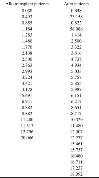
4.1. Bi-Pareto Model

The data as shown in Table 3 consist of 50 patients [9] with advanced acute myelogenous leukemia reported to the International Bone Marrow Transplant registry. 28 of these patients had received an autologous (auto) bone

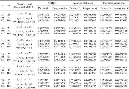
Table 1. AUROC, Mean absolute error and Root mean square error for Bi-Pareto model.

n m Parameters and

theoretical AUROC

AUROC Mean absolute error Root mean square error Parametric Non-parametric Parametric Non-parametric Parametric Non-parametric 25 50 100 25 50 100 1

λ =3, α1=2.5, 2

λ =1.5, α2=3 TAUROC = 0.943182

0.94510105 0.94328579 0.94380183 0.94243520 0.94332480 0.94305670 0.02369863 0.01700533 0.01235741 0.02987046 0.02083929 0.01457027 0.02966267 0.02133122 0.01531695 0.03753967 0.02603341 0.01807047 25 50 100 25 50 100 1

λ =3, α1=2.5, 2

λ=1.5, α2=3.5 TAUROC = 0.963182

0.96497062 0.96303781 0.96287246 0.96497062 0.96354760 0.96307080 0.01698465 0.01227429 0.00944949 0.02265412 0.01685340 0.01136324 0.02131398 0.01579954 0.01171875 0.02920274 0.02087816 0.01424524 25 50 100 25 50 100 1

λ =1.5, α1=3, 2

λ =1.5, α2=3 TAUROC = 0.5

0.49657810 0.50130506 0.49935328 0.50108800 0.50070400 0.50077890 0.05885142 0.04096787 0.02780156 0.07111360 0.04817280 0.03251370 0.07395279 0.05166748 0.03500349 0.08794395 0.05992312 0.04125929 25 50 100 25 50 100 1

λ =2, α1=2.2, 2

λ=1.7, α2=3.5 TAUROC = 0.781468

0.78773255 0.78368067 0.78395312 0.78146080 0.78318800 0.78081920 0.04923109 0.03399182 0.02350266 0.05214585 0.03607437 0.02663350 0.06064028 0.04236202 0.02924953 0.06570782 0.04505480 0.03335801 25 50 100 25 50 100 1

λ =1.5, α1=2, 2

λ=1.6, α2=3.5 TAUROC = 0.544207

0.54717102 0.54756388 0.54589646 0.56197280 0.56239600 0.56126120 0.06239505 0.04259772 0.02881548 0.07071822 0.04874452 0.03495051 0.07903727 0.05316711 0.03598686 0.08875004 0.06029191 0.04396757 25 50 100 25 50 100 1

λ =2, α1=2.2, 2

λ =2, α2=3.5 TAUROC = 0.614035

Table 2. AUROC, Mean absolute error and Root mean square error for Bi-two exponential model.

n m _{theoretical AUROC} Parameters and

AUROC Mean absolute error Root mean square error Parametric Non-parametric Parametric Non-parametric Parametric Non-parametric 25 50 100 25 50 100 1

θ =0.5,µ1=0.01, 2

θ =0.1, µ2=0.02 TAUROC = 0.815805

0.83499460 0.82622273 0.82298757 0.81624160 0.81504800 0.81738310 0.04208654 0.02831481 0.01880156 0.04988046 0.03440443 0.02551748 0.05264093 0.03502017 0.02334890 0.06202688 0.04261664 0.03188375 25 50 100 25 50 100 1

θ =0.9,µ1=0.04, 2

θ =0.1, µ2=0.09 TAUROC = 0.835128

0.86837326 0.85331447 0.84644056 0.85063360 0.84932000 0.85079500 0.04837996 0.03013549 0.01838186 0.05149320 0.03645040 0.02673079 0.05913404 0.03787997 0.02327638 0.06303793 0.04504823 0.03312037 25 50 100 25 50 100 1

θ =0.8,µ1=0.02, 2

θ =0.2, µ2=0.03 TAUROC = 0.789746

0.80805333 0.79925816 0.79494199 0.79181280 0.79055920 0.79057760 0.04655485 0.02924576 0.02015210 0.05028390 0.03642339 0.02597084 0.05751225 0.03615749 0.02494965 0.06243109 0.04553154 0.03279818 25 50 100 25 50 100 1

θ =1,µ1=0.02, 2

θ =0.5, µ2=0.04 TAUROC = 0.653063

0.65703285 0.66071741 0.65505433 0.65275680 0.65575840 0.65209930 0.05869804 0.03796614 0.02475642 0.06130676 0.04216340 0.02970049 0.07276215 0.04729011 0.03109102 0.07590817 0.05318708 0.03765384 25 50 100 25 50 100 1

θ =0.6,µ1=0.5, 2

θ =0.4, µ2=0.1 TAUROC = 0.852848

0.86134950 0.85599478 0.85436039 0.85224160 0.85211400 0.85307030 0.04053192 0.02858384 0.02046065 0.04318826 0.03142398 0.02176051 0.05006792 0.03560911 0.02524979 0.05545086 0.03911211 0.02740467 25 50 100 25 50 100 1

θ =0.7,µ1=1, 2

θ =0.4, µ2=0.3 TAUROC = 0.936809

0.93994355 0.93812690 0.93729421 0.93569280 0.93662200 0.93707370 0.02434545 0.01733529 0.01258346 0.02973861 0.02046246 0.01453632 0.03012846 0.02151211 0.01560085 0.03703009 0.02556071 0.01828934

Table 3. Leukemia free-survival times (in months) for Autologous and Allogeneic Transplants.

marrow transplant in which, after high doses of chemotherapy, their own marrow was reinfused to replace their destroyed immune system. 22 patients had an allogeneic (allo) bone marrow transplant where marrow from an HLA (Histocompatibility Leukocyte Antigen) matched sibling was used to replenish their immune systems.

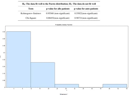
By using the easy fit software, it is seen that data in both groups fit well to the Pareto distribution. The p-values for Kolmogorov-Smirnov and Chi-square tests are shown in Table 4.

The histograms of Allo and Auto patients are shown in Figures 1 and 2.

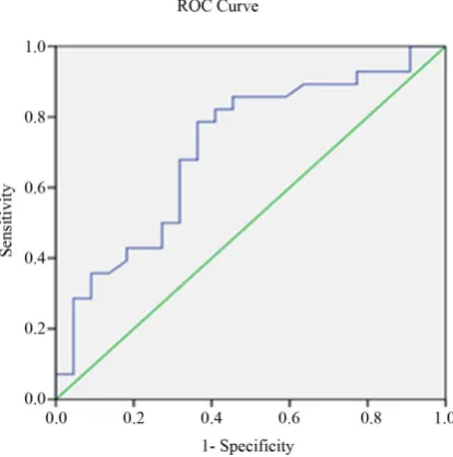
The area under ROC curve is calculated to be 0.711 by taking the allo patients as one group and auto patients as the second group when both groups follow Pareto distribution. The ROC curve is plotted in Figure 3.

For the above example, the parametric and non-parametric values of AUROC are 0.8164450 and 0.8049404 respectively. The root mean square errors for parametric and non-parametric approach are 0.2107548 and 0.2511394 respectively.

4.2. Bi-Two Parameter Exponential Model

Freireich [10] gave the results of a clinical trial of a drug 6-mercaptopurine (6-MP) versus a placebo in 42 chil- dren with acute leukemia and data is given in Table 5. The trial was conducted at 11 American hospitals. Those patients were selected who had a complete remission or partial remission of their leukemia induced by treatment with the drug prednisone. The trial was conducted by matching pair of patients at a given hospital by remission status (partial or complete) and randomising within the pair to either a 6-MP or placebo maintenance therapy. The patients were followed until their leukemia returned or until the end of the study (in months). The data are given below:

By using the easyfit software, we see that data for placebo and 6-MP patients fit well to the two parameter exponential distribution and this can also be concluded from the values in Table 6.

The histograms of Placebo and 6-MP patients are as shown in Figures 4 and 5.

Table 4. p-values for Kolmogrov-Smirnov and Chi-square tests.

H0: The data fit well to the Pareto distribution; H1: The data do not fit well

Tests p-value for allo patients p-value for auto patients

Kolmogorov-Smirnov 0.95568 (non-significant) 0.55822(non-significant) Chi-Square 0.88452(non-significant) 0.98721(non-significant)

Figure 2. Histogram for auto patients.

Figure 3. ROC Curve for the data given in Table 3.

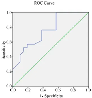
The area under ROC curve is calculated to be 0.759 by taking the placebo patients as one group and 6-MP pa- tients as the second group when both groups follow the two parameter exponential distribution. The ROC curve is plotted in Figure 6.

For the above example, parametric value of AUROC is 0.78713997 and non-parametric value is 0.45884774. The root mean square errors for parametric and non-parametric approach are 0.02813997 and 0.30015226 re- spectively.

5. Conclusion

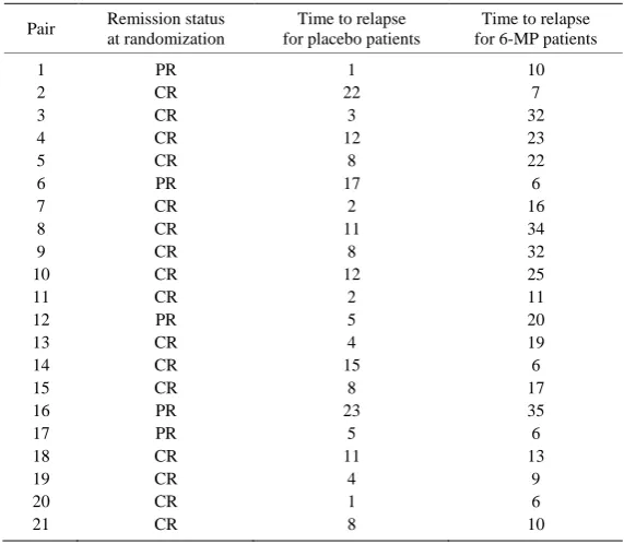
Table 5. Time to relapse for Placebo patients and 6-MP patients.

Pair Remission status at randomization

Time to relapse for placebo patients

Time to relapse for 6-MP patients 1

2 3 4 5 6 7 8 9 10 11 12 13 14 15 16 17 18 19 20 21

PR CR CR CR CR PR CR CR CR CR CR PR CR CR CR PR PR CR CR CR CR

1 22

3 12

8 17

2 11

8 12

2 5 4 15

8 23

5 11

4 1 8

10 7 32 23 22 6 16 34 32 25 11 20 19 6 17 35 6 13

9 6 10 CR: Complete Remission, PR: Partial Remission

Table 6. p-values for Kolmogorov-Smirnov and Chi-square tests.

H0: The data fit well to the two parameter exponential distribution;

H1: The data do not fit well.

Tests p-value for placebo patients p-value for 6-MP patients

Kolmogorov-smirnov 0.52283 (non-significant) 0.38267 (non-significant) Chi-Square 0.88355 (non-significant) 0.44643 (non-significant)

Figure 5. Histogram of 6-MP patients.

Figure 6. ROC Curve for the data given in Table 5.

root mean square and mean absolute errors are calculated using simulations. For both the models, the area under ROC curve can be estimated more accurately by parametric approach as compared to the non-parametric ap- proach. The applications have been discussed using real life data sets.

Acknowledgements

The first author is thankful to University Grants Commission, Government of India, for providing financial support for this work.

REFERENCES

[1] S. Satchell and W. Xia, “Parametrical Models of the ROC Curve: Applications to Credit Rating Model Validation,” Quantita-tive Finance Research Centre Research Paper 181, University of Technology, Sydney, 2006.

[3] D. Bamber, “The Area above the Ordinal Dominance Graph and the Area below the Receiver Operating Characteristic Graph,” Journal of Mathematical Psychology, Vol. 12, No. 4, 1975, pp. 387-415. http://dx.doi.org/10.1016/0022-2496(75)90001-2 [4] J. A. Hanley and B. J. McNeil, “The Meaning and Use of the Area under ROC Curve,” Radiology, Vol. 4, 1982, pp. 49-58. [5] D. M. Green and J. A. Swets, “Signal Detection Theory and Psychophysics,” Wiley, New York, 1966.

[6] A. P. Bradley, “The Use of the Area under ROC Curve in the Evaluation of Machine Learning Algorithms,” Pattern Recognition, Vol. 30, No. 7, 1997, pp. 1145-1159. http://dx.doi.org/10.1016/S0031-3203(96)00142-2

[7] N. L. Johnson and S. Kotz, “Continuous Univariate Distributions,” Vol. 1, Wiley, New York, 1970.

[8] S. J. Mason and N. E. Graham, “Area Beneath Relative Operating Characteristic (ROC) and Relative Operating Levels (ROL) Curve: Statistical Significance and Interpretation,” Quarterly Journal of the Royal Meteorological Society, Vol. 128, No. 584, 2002, pp. 2145-2166. http://dx.doi.org/10.1256/003590002320603584

[9] J. P. Klein and M. L. Moeschberger, “Survival Analysis Techniques for Censored and Truncated Data,” Springer-Verlag, New York, 2003.