A Taguchi method application for the part routing selection in Generalized Group Technology: A case Study

Munich Personal RePEc Archive

A Taguchi method application for the

part routing selection in Generalized

Group Technology: A case Study

Hachicha, Wafik and Masmoudi, Faouzi and Haddar,

Mohamed

Ecole Nationale d’ingénieurs de Sfax, Unité Modélisation Mécanique

et Production

17 December 2008

Online at

https://mpra.ub.uni-muenchen.de/12376/

4th _{International Conference on Advances in Mechanical Engineering and Mechanics ICAMEM2008}

16-18 December, 2008, Sousse, Tunisia

T

G

T

:

W. Hachicha

Unit of Mechanic, Modelling and Production (U2MP)

Higher Institute of Industrial Management of Sfax B.P. 954, 3018, Sfax, Tunisia

[email protected]

F. Masmoudi and M. Haddar

Unit of Mechanic, Modelling and Production (U2MP)

National Engineering School of Sfax, B.P.1173, 3038, Sfax, Tunisia

[email protected], [email protected]

Abstract

Cellular manufacturing (CM) is an important application of group technology (GT) that can be used to enhance both flexibility and efficiency in today’s small-to-medium lot production environment. The crucial step in the design of a CM system is the cell formation (CF) problem which involves grouping parts into families and machines into cells. The CF problem are increasingly complicated if parts are assigned with alternative routings (known as generalized Group Technology problem). In most of the previous works, the route selection problem and CF problem were formulated in a single model which is not practical for solving large-scale problems. We suggest that better solution could be obtained by formulating and solving them separately in two different problems. The aim of this case study is to apply Taguchi method for the route selection problem as an optimization technique to get back to the simple CF problem which can be solved by any of the numerous CF procedures. In addition the main effect of each part and analysis of variance (ANOVA) are introduced as a sensitivity analysis aspect that is completely ignored in previous research.

Keywords:Cellular Manufacturing, generalized Group Technology, route selection problem, Taguchi method, ANOVA, sensitivity analysis

1. Introduction

Cellular manufacturing (CM) has been one of the most successful ways that companies have used in order to cope with the challenges of today’s global competitive environment. CM is the implementation of Group Technology (GT) philosophy which determines and divides the parts into various families and the machines into cells by taking advantage of part similarity. The fundamental problem in CM is the cell formation (CF) problem which consist in identifying machine cells and part families.

different problems such as recommended by Hwang and Ree (1996) and Hachicha et al. (2008b). In addition, most of the existing CF methods in the presence of alternative routings (sequential iterative and simultaneous approaches) ignore the sensitivity analysis of alternative routings for each part. In other words, the drawback of these approaches is that information given by the remainder alternative routings for each part is not used after obtaining the CF solution. However, considering the competitive and the reactive nature of industry nowadays, an applicable approach should take the dynamic conditions into account. The approach developed in this paper addresses the first subproblem of CF with alternative routings. It attempts to determine the part routings while minimizing total intercellular part traffic. The originality of the present paper consists in using Taguchi method to the CF with alternative routings. Parts are considered as process parameters or factors and alternatives routings of each part as levels.

This manuscript is structured as follows. In section 2, the research methods based on Taguchi method and CF performances criteria which are proposed in literatureare briefly described. The proposed approach is then presented in Section 3 through a literature case study. Finally, concluding remarks and perspectives are made in Section 4.

2. Research Method

2.1. Taguchi method

The Taguchi method contains system design, parameter design, and tolerance design procedures to achieve a robust process and result for the best product quality (Taguchi, 1987). The purpose of system design procedure is to find the suitable working levels of the design factors. The parameter design procedure determines the factor levels that can generate the best performance of the product or process under study. The tolerance design procedure is used to fine-tune the results of parameter design by tightening the tolerance levels of factors that have significant effects on the product or process. In general, the parameter design of the Taguchi method utilizes orthogonal arrays (OAs) to minimize the time and cost of experiments in analyzing all the factors and uses ANOVA (analyse of variance) and the signal-to-noise (S/N) ratio to analyze the experimental data and find the optimal parameter combination. Using OAs significantly reduces the number of experimental configurations to be studied (Montgomery, 1991). Procedures for conducting a parameter design include the following steps:

1. Planning experiment

(1) Determine the control factors, noise factors and quality or performance measure responses of the product or process.

(2) Determine the levels of each factor.

(3) Select an appropriate orthogonal array (OA) table.

The selection of the most appropriate OA depends on the number of factors and interactions, and the number of levels for the factors. For examples: an L8 (27) OA can lay out 8 trials, up to 7 factors in

columns, and 2 factor levels. 2. Implementing experiment 3. Analyzing and examining result

(1) Determine the parameters signification (ANOVA)

(2) Conduct a main effect plot analysis to determine the optimal level of the control factors. (3) Execute a factor contribution rate analysis.

(4) Confirm experiment and plan future application.

2.2. Cell formation performances criteria

those CF criteria is that the final solution must be performed for the calculation of those performance criteria. Therefore, they cannot be used as response measure for the proposed Taguchi method application. To overcome this condition, we suggest the use of another criterion which must put forward automatically the quality of a CF solution without performing the diagonal blocs form (as presented by Hachicha et al. (2008a)). This criterion which will be presented in the following subsection can be applied to the initial incidence part-machine matrix.

The initial incidence matrix which is called by A is a binary matrix which rows are parts and columns stand for machines. Since CF problem is considered as a dimension reduction problem in which a large number of interrelated machines and parts are grouped into a smaller set of independent cells, the principal components analysis application can give rapidly an excellent solution as mentioned by (Albadawi et al. 2005) and (Hachicha et al. 2006). Principal components analysis consists of determining a small number of principal components that recover as much variability in the data as possible. These components are linear combinations of the original variables and account for the total variance of the original data. Thus, the study of principal components can be considered as putting into statistical terms the usual developments of eigenvalues and eigenvectors for positive semi-definite matrices. The eigenvector equation where the terms λ₁≥λ₂≥...≥λ_m are the real, nonnegative roots of the determinant polynomial of degree m given as:

i

det(S-λ I)=0 ; i∈<1,m> (1)

Where m: denote the number of machines and S: the covariance matrix which is expressed by:

B B p 1

S= t (2)

Where B: denote the standardization matrix of the initial incidence matrix A, Bt: denote the transpose of matrix B, and p: the number of parts. When principal components analysis was performed on the mean centred data, a model with the first and the second principal components was usually obtained. This model explained the recover Cumulated Percentage (CP) of the variance in the data by the following expression:

1 2 1 2 m

k k 1

λ λ λ λ

C P

m

λ

=

+ +

= =

∑

(3)

Detailed description of principal components analysis application in cell formation problem and CP calculation can be found in Hachicha et al. (2008a). The CP as statistical criterion measure is available by using one of several commercial software packages including SAS, SPAD, SPSS, S-PLUS, XLSTAT, and others.

3. The proposed methodology

The aim of this case study is to determine the best part routings of each part type using Taguchi method while minimizing CP measure et consequently the total intercellular part traffic. As mentioned in the preceding section, the Taguchi method contains principally three steps which are detailed in the following subsections. It should be noted that S/N ratio is not performed because the target is fixed and signal factors are absent (static design).

3.1. Orthogonal array experiments

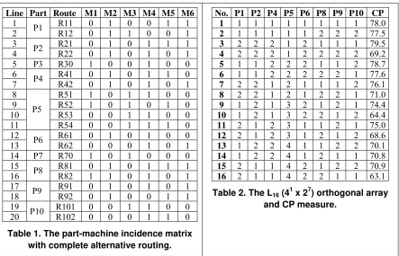
R52, R53 and R54). Part P3 and P7 have not alternatives routing. This example is taken from (Sankaran and Kasilingam, 1990). The machine-part matrix with complete set of alternative routes is shown in Table 1. The first subproblem consists of selecting one route for each part will give the best CP as the adopted performance measure criteria for grouping of the machines in cells. As explained in subsection 2.1, optimizing a process design means determining the best architecture levels of each factors (i.e. in this case, determining the best route of each parts).

The selection of routings affects the CF final solution and consequently the CP measure which is considered as the output quality response of the proposed Taguchi method application. The example of Table 1 contains ten parts including two fixed routing parts which are P3 and P7. Therefore, eight process parameters were identified. Part P5 with 4 levels and each other with two levels. The orthogonal array (OA), L16 (41 x 27), is used to conduct ideally the experiment in this example. In fact,

it can lay out 16 trials, up to 8 factors in columns: 7 factors with 2 levels each one and only one factor with 4 levels. It should be noted that this OA reduces the number of factorial design experiments 512 (41 x 27) to only 16 experimental evaluations. The layout of the L16 (41 x 27) OA is shown in Table 2.

It also shows the output responses (CP measure) for each experimental trial (configuration).

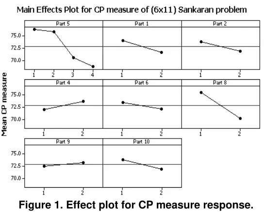
3.2. Implementing experiments and Main effect plot

Due to the deterministic aspect of the problem, one trial was conducted for each configuration. Then the main effect plot is analyzed to set the optimal route for each part. Afterward, analysis of main effect is applied as a sensitivity analysis to determine each part signification. The MINITAB 14.0 software is used to assist the interpretation of the results.

Line Part Route M1 M2 M3 M4 M5 M6

1 R11 0 1 0 0 1 1

2 P1 R12 0 1 1 0 0 1

3 R21 0 1 0 1 1 1

4 P2 R22 0 1 0 1 0 1

5 P3 R30 1 0 0 1 0 0

6 R41 0 1 0 1 1 0

7 P4 R42 0 1 0 1 0 1

8 R51 1 0 1 1 0 0

9 R52 1 0 1 0 1 0

10 R53 0 0 1 1 0 0

11 P5

R54 0 0 1 1 1 0

12 R61 0 1 0 1 0 0

13 P6 R62 0 0 0 1 0 1 14 P7 R70 1 0 1 0 0 0

15 R81 0 1 0 1 1 1

16 P8 R82 1 1 0 1 0 1

17 R91 0 1 0 1 0 1

18 P9 R92 0 1 0 0 1 1

19 R101 0 0 1 1 0 0

20 P10 R102 0 0 0 1 1 0

Table 1. The part-machine incidence matrix with complete alternative routing.

No. P1 P2 P4 P5 P6 P8 P9 P10 CP

1 1 1 1 1 1 1 1 1 78.0

2 1 1 1 1 1 2 2 2 77.5

3 2 2 2 1 2 1 1 1 79.5

4 2 2 2 1 2 2 2 2 69.2

5 1 1 2 2 2 1 1 2 78.7

6 1 1 2 2 2 2 2 1 77.6

7 2 2 1 2 1 1 1 2 76.1

8 2 2 1 2 1 2 2 1 71.0

9 1 2 1 3 2 1 2 1 74.4

10 1 2 1 3 2 2 1 2 64.4

11 2 1 2 3 1 1 2 1 75.0

12 2 1 2 3 1 2 1 2 68.6

13 1 2 2 4 1 1 2 2 70.1

14 1 2 2 4 1 2 1 1 70.8

15 2 1 1 4 2 1 2 2 70.9

16 2 1 1 4 2 2 1 1 63.1

Table 2. The L16 (41 x 27) orthogonal array and CP measure.

3.3. Analyzing and examining result (ANOVA)

In this work, ANOVA is used as a sensitivity analysis to determine the alternative parts effects. ANOVA analysis for estimating the error variance for each part effect and the variance of the prediction error is given in Table 3. There is a statistical test which is called F value test for determining the significant factors. F value is a test for comparing model variance with residual (error) variance. When the variances are close to each other, the parts have a significant effect on the CP response. F value is calculated by term mean square divided by residual mean square. “Prob > F” is the probability of seeing the observed F value if the null hypothesis is true (there is no part effect). If the “Prob > F” value is very small (less than 5 %) then the individual terms in the model have a significant effect on the response.

Precision of a parameter estimate is based on the number of independent samples of information which can be determined by degree of freedom (DOF). The DOF equals to the number of experiments minus the number of additional parameters estimated for that calculation. The sum of squares values due to various parts, tabulated in the third column of Table 3, are a measure of the relative importance of the factors in changing the values of recovery. The mean square for a factor is computed by dividing the sum of squares by the DOF.

Part DOF Sum of Mean F p-value prob.> Signification

P1 1 22.80 22.80 2.51 0.17 No

P2 1 13.87 13.87 1.52 0.27 No

P4 1 10.72 10.72 1.18 0.32 No

P5 3 171.91 57.30 6.30 0.04 Significant

P6 1 6.63 6.63 0.73 0.43 No

P8 1 107.64 107.64 11.83 0.02 Significant

P9 1 1.89 1.89 0.21 0.66 No

P10 1 13.87 13.87 1.52 0.27 No

Residual 5 45.51 9.10

Total 15

Table 3. The ANOVA table of mean CP measure

The ANOVA indicates that for the CF solution performance measure of the case study, the parts P5 and P8 are the most significant and consequently the most sensitivity effect to the CF final solution.The others parts P9, P6, P4, P2, P10 and P1 have insignificant effect on the CP measure. The final step is to confirm the validity of the CP measure using the optimal route selection of each part.

Indeed, this validation experiment yield a CP result of 82.1 %, which is better than each value depicted in Table 2.

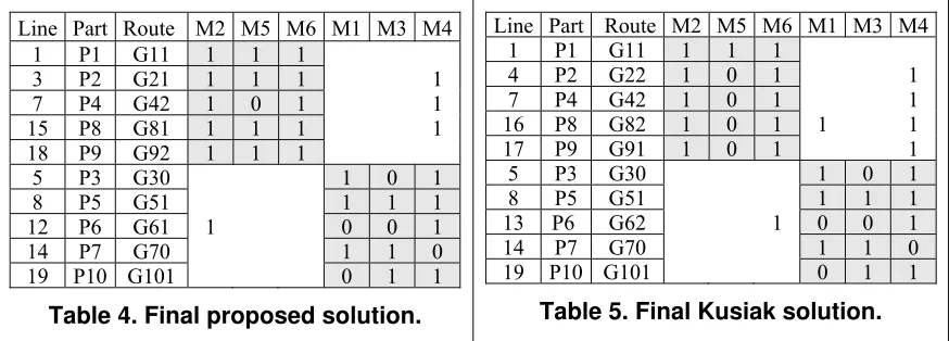
Comparing the result in Table 4 with the result in Table 5, it is noted that the proposed Taguchi method application has provided a better solution than Kusiak’s solution. In fact, the proposed solution presents only 4 exceptional elements and 6 void elements while final Kusiak’s solution provides 6 exceptional elements and 8 void elements. It should be noted that, both proposed solution and Kusiak’s solution gives same cells configuration: cell 1 consists of machines 2, 5 and 6 while cell 2 consists of machines 1, 3 and 4. In addition, cell 1 contains parts 1, 2, 4, 8 and 9 while cell 2 contains parts 3, 5, 6, 7 and 10.

Line Part Route M2 M5 M6 M1 M3 M4

1 P1 G11 1 1 1

3 P2 G21 1 1 1 1

7 P4 G42 1 0 1 1

15 P8 G81 1 1 1 1

18 P9 G92 1 1 1

5 P3 G30 1 0 1

8 P5 G51 1 1 1

12 P6 G61 1 0 0 1

14 P7 G70 1 1 0

19 P10 G101 0 1 1

Table 4. Final proposed solution.

Line Part Route M2 M5 M6 M1 M3 M4

1 P1 G11 1 1 1

4 P2 G22 1 0 1 1

7 P4 G42 1 0 1 1

16 P8 G82 1 0 1 1 1

17 P9 G91 1 0 1 1

5 P3 G30 1 0 1

8 P5 G51 1 1 1

13 P6 G62 1 0 0 1

14 P7 G70 1 1 0

19 P10 G101 0 1 1

Table 5. Final Kusiak solution.

4. Conclusion

In this study we have used Taguchi method as an optimization technique in cellular manufacturing systems design. The objective is to solve the route selection problem for the cell formation with alternative routings. Furthermore, mean effect analysis and analysis of variance can provide a sensitivity analysis which is completely ignored in previous CF approach. The present approach can be applied to other problems that include large number of machines, parts and routings. Proving the effectiveness and the efficiencies of the proposed approach is our interesting research perspective.

References

Albadawi, Z., Bashir, H. A., Chen, M., (2005). A mathematical approach for the formation of manufacturing cell, Computers

and Industrial Engineering, 48, 3-21.

Caux, C., Bruniaux, R., Pierreval, H., (2000). Cell formation with alternative process plans and machine capacity constraints: A new combined approach. Int. J. of Production Economics, 64, 279–284.

Gupta, T., (1993). Design of manufacturing cells for flexible environment considering alternative routings, Int. J. of

Production Research, 31(6), 1259-1273.

Hachicha, W., Masmoudi, F. and Haddar, M. (2006). A correlation analysis approach of cell formation in cellular manufacturing system with incorporated production data. Int. J. of Manufacturing Research, 1(3), 332–353.

Hachicha, W., Masmoudi, F., and Haddar, M. (2008a). Formation of machine groups and part families in cellular manufacturing systems using a correlation analysis approach. Int. J. of Advanced Manufacturing Technology, 36, (11-12), 1157-1169

Hachicha, W., Masmoudi, F., and Haddar, M. (2008b). Combining Axiomatic Design and Designed Experiments for cellular manufacturing systems design framework. Int. J. of Agile systems and Management, 3(3-4), paperin print

Hwang, H., Ree, P. (1996). Routes selection for the cell formation problem with alternative part process plans. Computers

and Industrial engineering, 30(3), 423-431.

Kusiak, A., (1987). The generalized group technology concept. Int. J. of Production Research, 25, 561-569. Montgomery, D.,C. (1991). Design and Analysis of Experiments, ed. John Wily, New York

Nagi, R., Harhalakis, G., Proth, J. (1990) Multiple routings and capacity considerations in Group Technology applications,

Int. J. of Production Research, 28(12), 2243-2257

Sankaran, S., Kasilingam, R. (1990). An integrated approach to cell formation and part routing in Group Technology manufacturing system. Engineering Optimization, 16, 235-245.

Taguchi, G. (1987). System of Experimental Design, Unipub/Kraus, International Publication.