Reaction curves

Munich Personal RePEc Archive

Reaction curves

Giocoli, Nicola

University of Pisa, Department of Economics

2008

Online at

https://mpra.ub.uni-muenchen.de/33809/

REACTION CURVES

Basic concepts

A reaction curve RC, also called reaction function or best-reply function, is the locus of optimal,

i.e. profit-maximizing, actions R a_i

( )

_j that a firm i may undertake for any given action a_j chosen

by a rival firm j. The RC diagram is the standard tool for the graphical analysis of duopoly. In the

diagram the market equilibrium is at the intersection of the RCs, one for each firm. The commonest

case of RC diagram is that of the Cournot duopoly model.

Consider two firms 1 and 2 producing a homogeneous product with output levels q₁ and q₂ and

aggregate output Q=q₁+q₂. Provided invertibility conditions are met, the inverse demand function

gives the market price associated with aggregate output p Q

( )

= p q

(

₁+q₂

)

. Assume each firm has a

cost function c q_i

( )

_i , i=1, 2, and take the strategic variable for both firms to be the output level, so

that firm 1’s maximization problem is:

(

)

( )

( )

1 1 1 2 1 1 1

maxq

π

q q, = p Q q −c q . Given that firm 1’s

profit also depends on firm’s 2 output, firm 1’s optimal choice must also take into account firm 2’s choice. A similar problem can be formulated for firm 2.

Following the so-called Cournot assumption, we model each firm as taking as given the rival’s quantity. The first order condition (FOC) for each firm is therefore:

(

)

( )

( )

( )

1, 2

0

i

i i i i

q q

p Q p Q q c q q

π

∂

′ ′

= + − =

∂ , i=1, 2

Firm 1’s FOC determines the optimal, i.e., profit-maximizing, output choice by firm 1 as a function of either its belief about firm 2’s expected output choice or its observation of firm 2’s actual choice (see below for an explanation of these two possible interpretations). As in Cournot (1971 [1838], Fig.2), we depict the pair of FOCs with the RC diagram, where the RC of firm 1 (RC1) is implicitly

defined by the FOC 1

(

1

( )

2 2

)

1

,

0 R q q

q

π

∂

=

∂ , and that of firm 2 (RC2) by

( )

(

)

2 2 1 1

2

,

0 R q q

q

π

∂

=

∂ . The

name reaction curve captures the idea that a firm will optimally modify its choice following the change in its belief about (or its observation of) the rival’s choice. The slope of each RC indicates the size of a firm’s optimal reaction to such a change. For example, the slope of RC1 is:

( )

2 1

1 2

1 2 2

1 2 1 q q R q q

π

π

∂ ∂ ∂ ′ = − ∂ ∂

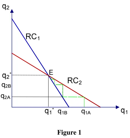
The diagram below is based on the simplifying assumption of linear demand and constant and identical marginal cost (see Fulton 1997, Martin 2002 for a step-by-step derivation of the diagram).

In such a case the RCs are straight lines with negative slope. The equilibrium pair

(

q q₁*, *₂

)

lies at

[image:3.595.179.408.162.405.2]

the intersection of the RCs.

Figure 1

Two interpretations

In the belief-based version of the model, two conditions need be satisfied for the firms’ choices to constitute an equilibrium (Kreps 1990). First, no firm, on the basis of its own beliefs, must wish to modify its own choice. Second, the firms’ equilibrium actions must be consistent with the beliefs upon which they act. Hence, a Cournot equilibrium in a basic duopoly model is given by the output

pair

(

q q1*, *2

)

such that: i) each firm is choosing its profit maximizing output given the beliefs about

the other firm’s choice, and, ii) each firm’s beliefs are correct at equilibrium. The similarity with the game-theoretic notion of Nash equilibrium, and with the static fixed point concept underlying it, is well-known. Yet, the association with non-cooperative game theory came just with Shubik 1959.

Before that, Cournot model was mostly considered as a dynamic analysis involving a sequential adjustment process undertaken by two firms who ignored that their own choices could influence the rival’s behavior. The outcome of the process – the equilibrium position – was viewed as the end state of a trial-and-error sequence of actual output choices along the RCs. An instance of such a sequence is showed in the diagram above. Assume firm 2 observes output q_1A chosen by firm 1. Its

profit-maximizing reaction to the rival’s choice may be read on RC2 and amounts to producing q2A.

The process actually converges to equilibrium (more on this convergence below), i.e., to the pair

(

* *

)

1, 2

q q such that neither firm has any further incentive to modify its own choice.

The dynamic reading of Cournot model is highly questionable because it requires the two firms to adopt a myopic, almost irrational behavior. As William Fellner put it, at equilibrium the duopolists turn out to be <<… right for the wrong reasons.>> (1949, p.58). Each firm is in fact assumed to go on making its output choice by always taking as given the rival’s quantity – this despite the evidence clearly showing that the rival is actually reacting to one’s own choice. Indeed, the only consequence of the rival’s reaction is taken to be the modification of the quantity that each firm still

takes as given in its own RC. Though not 100% faithful to Cournot’s own words (he actually assumed that duopolists only looked at the direct influence of each other’s output choices, while disregarding the indirect ones – viz., the reactions – because that would demand too much from their reasoning power: see Giocoli 2003), the interpretation of RCs as the illustration of a myopic sequence of actual actions and reactions has been dominant in the first half of the 20th century, starting at least from Fisher 1898.

However, also the belief-based version of Cournot model has a long history. As early as 1924 Arthur Bowley argued that in order to solve the FOCs of a standard duopoly problem <<...we

should need to know [q₂] as a function of [q₁], and this depends on what each producer thinks the other is likely to do. >> (Bowley 1924, 38). A new notion, the conjectural variation v_{i j} = ∂q_i ∂q_j,

1, 2

i= , was introduced, to represent firm i’s arbitrary conjecture about how its rival j would respond to a (small) variation of i’s output. The conjectural variation then entered both FOCs to highlight the fact that the solution of the duopoly model should depend upon the exact value of each firm’s conjecture over the rival’s reaction. The Cournot model became just a special case – that with v₁₂ =v₂₁ =0, to indicate that each firm’s believed the rival would not react to its own choice –

but an infinite array of v_{i j} values was equally possible. A stream of literature elaborated Bowley’s

intuition, to emphasize the intrinsic indeterminacy of duopolistic interaction.

game each RC indicates what a firm would do in case it happened to know of a change in the rival’s action, which of course it does not because no RC point outside the Nash equilibrium can ever be observed. Therefore, if we stick to the actual-choice interpretation of Cournot competition even in a simultaneous setup, we must admit that the construction of the RC diagram is a mere technical device, only used for expositional purposes. On the contrary, actual-choice RCs have a real economic content in the dynamic setup typical of sequential games. The RC may now be read as a function determining a firm’s (myopic) reaction in a given period in terms of the other firm’s action during the preceding period; moreover, each firm may well exploit the rival’s RC to calculate how a change in its behavior may affect the rival’s (myopic) choice.

Extensions

The simple, textbook version of the RC diagram enjoys some useful properties. Assuming quantity competition, a linear inverse demand and constant marginal costs, the RCs are straight lines with constant negative slopes and intercepts with the axis equal to, respectively, the perfectly competitive and the monopoly quantities (see figure 2).

Figure 2

Consider RC1 and adopt for definiteness the actual-choice interpretation. RC1’s intercept with the X-axis identifies the optimal choice when q₂ =0, i.e., when firm 1’s residual demand (the demand

left after firm 2 has chosen its output level) coincides with market demand. But when firm 1 faces the whole demand curve, its optimal choice is to produce the monopoly quantity q_m. Conversely,

happen when q₂ is so large to push market price down to equal the common average and marginal

cost, i.e., when firm 2 offers the perfectly competitive quantity q_pc (because in such a case any

positive output by firm 1 would push price further down, below cost). A similar argument explains the intercepts of RC2.

Given that q_pc is larger than q_m, it follows that whenever q₁ is measured on the X-axis RC1

always crosses RC2 from above. This, in turn, warrants the stability of Cournot equilibrium as implemented through the above-mentioned trial-and-error process. Remarkably, Cournot himself acknowledged that, though stability might not be warranted in general, it was actually implied by the relative size of RCs’ intercepts (1971, 81-2). In a more general setting, the equilibrium may either be nonexistent or multiple (see Martin 2002). A non-existence result may emerge when RCs are discontinuous (as in Amoroso 1921’s counterexample or because firms’ profit functions are not concave due to the “excessive” convexity of demand). Multiplicity may ensue when the slope of the RCs (say, of R q₁′

( )

₂ ) is larger than 1 in absolute value. Both cases are obviously excluded in the

standard, linear version of the model.

Figure 2 also shows a simple graphical technique for comparing the market performance of a Cournot equilibrium with that of the two extreme cases, monopoly and perfect competition. Given

the RCs’ intercepts with the axes, we may draw a dashed line representing the

(

q q1, 2

)

pairs that

jointly give the perfectly competitive output q_pc and a dotted line for the pairs giving the joint

monopoly output q_m. The two lines allow an immediate understanding of the intermediate nature

of the Cournot equilibrium pair

(

* *

)

1, 2

q q : total output q_d =q₁*+q*₂ is lower than q_pc and larger than

m

q . It follows that the price level and the firms’ profit are also intermediate between those in the

two extreme cases.

The standard RC diagram may also encompass the case of a difference in the firms’ efficiency. The thick line in Figure 2 is RC2bis , that is, firm 2’s RC when it enjoys a cost advantage over firm 1. RC2bis is higher because firm 2 optimally produces more than before for any quantity offered by firm 1. Hence, also q*₂ will be larger (and q₁* smaller) than in the traditional Cournot equilibrium.

Finally, take the most general form of the slope of the RC, namely,

( )

2 1

1 2

1 2 2

1 2 1

a a R a

a

π

π

∂

∂ ∂ ′ = −

∂ ∂

, where

i

maximum profit requires

2 1 2 1

0

a

π

∂ <

∂ , it turns out that the sign of R a1′

( )

2 depends on that of the

cross partial derivative of firm 1’s profit function, i.e., on how

π

₁ varies as an effect of a change in the rival’s action. RC1 is negatively sloped when, as in the Cournot model, the cross partial

2 1

1 2

a a

π

∂

∂ ∂ is negative and positively sloped when it is positive. In the former case, firms’ actions are

[image:7.595.175.415.244.480.2]

said to be strategic substitutes (e.g. quantities), in the latter, strategic complements (e.g. prices; see Bulow et al. 1985).

Figure 3

The RC diagram for the case of strategic complements is therefore as in figure 3, which represents two firms competing in prices and producing a homogeneous product (so-called “pure

Bertand” case). The equilibrium price pair is

(

p_pc,p_pc

)

, where p_pc is the perfectly competitive

price, namely a price equal to marginal cost c. In case of partial product differentiation, both RCs

would shift upward and the equilibrium pair

(

p p1*, *2

)

would lie somewhere between the

competitive and the monopoly price pairs. If the differentiation is complete, the RCs become orthogonal to the axes, with intercepts at the monopoly price p_m, to suggest the independence of

each firm’s price decision from the rival’s choice.

Nicola Giocoli

References

Amoroso L. 1921, Lezioni di Economia Matematica, Bologna: Zanichelli

Bowley A.L. 1924, The Mathematical Groundwork of Economics, Oxford: OUP.

Bulow J. Geanakoplos J. and Klemperer P.D. 1985, “Multimarket oligopoly: strategic substitutes and complements”, Journal of Political Economy 93 (3), 488-511

Cournot A.A. 1971 [1838], Researches into the Mathematical Principles of the Theory of Wealth, New York: Augustus M. Kelley Publishers.

Fellner W. 1949, Competition among the few, New York: A.A. Knopf.

Fisher I. 1898, “Cournot and mathematical economics”, Quarterly Journal of Economics, 12, 119-138.

Friedman J. 1977, “Cournot, Bowley, Stackelberg and Fellner, and the evolution of the reaction function”, in: Balassa B. & Nelson R. (eds.), Economic Progress, Private Values and Public Policy: Essays in Honor of William Fellner, Amsterdam: NorthHolland, 139-160.

Fulton M. 1997, “A graphical analysis of the Cournot-Nash and Stackelberg models”, Journal of Economic Education, 28 (1), 48-57.

Giocoli N. 2003, “Conjecturizing Cournot: the conjectural variations approach to duopoly theory”,

History of Political Economy, 35 (2), 175-204

Kreps D. 1990, A Course in Microeconomic Theory, Harvester-Wheatsheaf.

Martin S. 2002, Advanced Industrial Economics. Second Edition, Oxford: Blackwell