Munich Personal RePEc Archive
Conditional RD Subsidies
Atallah, Gamal
University of Ottawa
2007
Online at
https://mpra.ub.uni-muenchen.de/2895/
DÉPARTEMENT DE SCIENCE ÉCONOMIQUE DEPARTMENT OF ECONOMICS
CAHIERS DE RECHERCHE & WORKING PAPERS
# 0702E
Conditional R&D Subsidies
by Gamal Atallah
University of Ottawa
ISSN: 0225-3860
CP 450 SUCC. A P.O. BOX 450 STN. A
OTTAWA (ONTARIO) OTTAWA, ONTARIO
Abstract
This paper introduces a new type of R&D subsidy, which is conditional on the success of the R&D project. In a three-stage model, the government chooses a subsidy(ies) in the first stage; in the second stage, a monopolist chooses R&D effort which determines the size or the probability of success of the R&D project; in the last stage, the firm chooses its output. It is found that conditional subsidies can yield the same level of innovation and welfare as unconditional subsidies. However, when the probability of success is sufficiently low (be it endogenous or exogenous), conditional subsidies yield suboptimal levels of innovation and welfare. When the firm chooses the probability of success, conditional subsidies can have the advantage of a lower expected cost of the subsidy to the government. I consider the simultaneous use of conditional and unconditional subsidies, and show that different combinations of the two can lead to the same levels of innovation and welfare as unconditional subsidies alone. Finally, reverse conditional subsidies, which the firm gets only if the project fails, are considered. It is found that they yield the same level of innovation as unconditional subsidies, except when the probability of success is sufficiently high. Comparing conditional subsidies with reverse conditional subsidies, conditional subsidies yield higher (lower) welfare when the probability of success is high (low).
Keywords: R&D subsidies, Innovation, R&D policy, Innovation policy JEL codes: L12, L52, O31, O38
Sommaire
Cet article présente un nouveau type de subvention à la R&D, qui est fonction du succès du projet de recherche. Dans un modèle à trois étapes, le gouvernement choisit une/des subvention(s) à la première étape; à la deuxième étape, un monopoleur choisit la taille du projet ou la probabilité de succès; à la dernière étape, la firme choisit son output. Les subventions conditionnelles peuvent générer les mêmes niveaux d'innovation et de bien-être que les subventions non-conditionnelles. Cependant, lorsque la probabilité de succès est suffisamment faible (qu’elle soit endogène ou exogène), les subventions conditionnelles produisent des niveaux d'innovation et de bien-être sub-optimaux. Lorsque la firme choisit la probabilité de succès, les subventions conditionnelles peuvent avoir l'avantage d'un coût attendu inférieur pour le gouvernement. On considère l'utilisation simultanée des subventions conditionnelles et non-conditionnelles, et l’on montre que plusieurs combinaisons des deux peuvent produire les mêmes niveaux d'innovation et de bien-être que les subventions non-conditionnelles. Finalement, des subventions conditionnelles que la firme obtient seulement si le projet échoue, sont considérées. Ces subventions génèrent le même niveau d'innovation que les subventions non-conditionnelles, sauf lorsque la probabilité de succès est suffisamment élevée. Comparant les subventions conditionnelles reliées au succès et celles reliées à l’échec, on trouve que celles reliées au succès génèrent un niveau de bien-être supérieur (inférieur) lorsque la probabilité de succès est élevée (faible).
1
I would like to thank the participants in the EARIE conference (Porto) for useful comments.
2There is also the possibility that even failed R&D projects are useful in that the human capital built from such
projects is transferred to other firms through employee mobility. Although MNen (2004) finds little support for this hypothesis using Norwegian data.
3
In Finland, during the evaluation of subsidy provision, R&D projects are classified based on several criteria. One of these criteria is the risk associated with the R&D project; the projects are ranked from 0 to 5, with 0 representing the “no 1. Introduction1
R&D subsidies are used by governments to encourage firms to increase their investments in
R&D. R&D subsidies are the fastest growing and second largest type of government aid to industry
in developed countries (Nevo, 1998). R&D subsidies are the subject of a large economic literature.
Examples are Petrakis and Poyago-Theotoky (2002), Busom (2000), Klette et al. (2000), Ekholm
and Torstensson (1997), and Davidson and Segerstrom (1998). While a variety of forms of R&D
subsidies have been studied, a common feature of those subsidies is that they are unconditional, that
is, their provision or their level is not related to the technical or commercial success of the research
project.
Yet, there may be benefits to relating the provision of a R&D subsidy, or its level, to the
success/failure of a R&D project, or to the level of risk associated with the project. Such a scheme,
by rewarding success, may induce firms to perform better research, to increase the chances of
success of the project and/or the quality of the outcome. Moreover, with firms having different
research capabilities, R&D subsidies linked to success may select the best firms, and eliminate those
performing the least successful research. Making financing conditional on success can reduce
adverse selection and moral hazard (Aghion and Howitt, 1998). With limited government funds
available for subsidies, it may make sense to allocate those budgets to the best R&D projects and
to the best performers.2
Empirically, there is evidence that some countries incorporate some form of conditionality
into their support for R&D. Tanayama et al. (2004) find that in Finland, R&D subsidies are
increasing in technical challenge; this can be interpreted as a policy whereby the government allows
higher R&D subsidies to more risky or difficult projects.3 Fölster (1991) analyzes the different types
of R&D subsidies in use. One type of R&D support is a loan that is repaid to the government only
if the R&D project is successful. This is equivalent to a R&D subsidy based on failure; this
4The tax system may contain hidden conditionalities. For instance, the corporate income tax coupled with a
(unconditional) tax incentive for R&D incorporates an implicit conditional subsidy (which the firm keeps only if the project fails), since greater technological and commercial success imply a higher repayment rate.
5
Mansfield et al. (1977) identify three types of success probabilities: technical completion (0.57), commercialization given technical completion (0.65), and financial success given commercialization (0.74). The numbers in brackets represent those probabilities for 16 firms operating in the chemical, pharmaceutical, electronics, and petroleum industries. These numbers show that the probability of failure is significant.
which are paid to the government based on the sales form the invention; hence, the higher the
(commercial) success of the project, the lower is the real subsidy rate. Or, the government, in
exchange for the subsidy, receives a stock option which can be exercised if the stock value rises
significantly, i.e., if the project is commercially successful. Moreover, based on a sample of Swedish
firms, Fölster finds that “selective” subsidies (such as royalty grants, conditional loans and stock
options) induce more additional private R&D than more traditional subsidies, such as tax incentives,
project grants and project loans. In France, the Agence nationale de valorisation de la recherche
provides innovation support which is reimbursed if the project succeeds (Guellec, 2001), which
amounts to a subsidy based on failure. Technology Partnerships Canada, a program aimed at
providing seed money to promote innovation in automotive, aerospace, defense and high-tech
companies, incorporates repayment of royalties based on commercial success. Until 1996, Australian
firms benefited from a higher deduction rate for R&D expenditures when the investments were fully
at risk (Department of Finance Canada, 1997).
Given that some form of conditionality in the support of R&D is being used by several
countries,4 there is a gap in the economic literature, which is the study of the properties and
consequences of such conditional subsidies. To fill this gap in our understanding of the impact of
R&D policies, this paper proposes a R&D subsidy which is conditional upon the success of the
project: if the R&D project succeeds, the firm obtains the subsidy; if the R&D project fails, the firm
has to cover all the expenses itself.5 Moreover, the simultaneous use of conditional and
unconditional R&D subsidies is considered. Finally, I consider the use of reverse conditional R&D
subsidies, where the firm has to pay the subsidy back to the government (or, equivalently, does not
get the subsidy) in case of success of the project. The logic behind such a subsidy is that if the
project fails, the firm may not have the means to pay the subsidy back. If the project succeeds,
however, the firm benefits commercially, and has the financial ability of paying back the subsidy.
6
Tassey (1996) discusses the use of tax incentives vs. direct funding to deal with different types of technological and commercial risks, but does not discuss conditional funding.
To consider these issues, the paper adopts a three-stage framework. The government chooses
a subsidy(ies) in the first stage; in the second stage, a monopolist chooses R&D effort which
determines the size of the R&D project or the probability of success of the project; in the last stage,
the firm chooses its output. It is found that conditional subsidies can yield the same level of
innovation and welfare as unconditional subsidies. However, when the probability of success is
sufficiently low (be it endogenous or exogenous), conditional subsidies yield suboptimal levels of
innovation and welfare. When the firm chooses the probability of success, conditional and
unconditional subsidies yield the same levels of innovation and welfare, but conditional subsidies
can have the advantage of a lower expected cost of the subsidy to the government. I consider the
simultaneous use of conditional and unconditional subsidies, and show that different combinations
of the two can lead to the same levels of innovation and welfare as unconditional subsidies alone.
Finally, reverse conditional subsidies yield optimal levels of innovation and welfare, except when
the probability of success is sufficiently high. Comparing conditional subsidies with reverse
conditional subsidies, conditional subsidies yield higher (lower) welfare when the probability of
success is high (low). In all, eight different models are considered, allowing for different policy
instruments (conditional and/or unconditional subsidies) and different choices of innovation effort
by the firm (innovation size versus probability of success); more specifically, for each choice
variable by the firm, four combinations of policy instruments are considered: unconditional subsidies
only, conditional subsidies only, conditional and unconditional subsidies together, and reverse
conditional subsidies only.
There is a small literature on R&D uncertainty. Poyago-Theotoky (1998) analyses the role
of a public firm in a mixed duopoly under uncertainty. Miyagiwa and Ohno (2002) analyze
cooperative R&D in an oligopoly with spillovers and uncertainty. Lambertini (2004) studies the
impact of demand uncertainty on R&D. However, the interaction between uncertainty and R&D
subsidization has not been analyzed.6
7
In a duopoly setting with spillovers, Helm and Schöttner (2004) consider an output subsidy given to the firm that develops the best technology. They find that such a subsidy can induce under or over-investment in R&D relative to a general output subsidy.
8
He goes even further, suggesting that risky investments should be subsidized, while safer investments should be taxed. This is because in his model, when firms choose the probability of success, they invest too much in safe projects. Patents are granted only to a successful innovation, and hence constitute a conditional reward.7
Lakdawalla and Sood (2004) distinguish between patents and prizes, which constitute a conditional
reward, and research subsidies, which are unconditional. They show that inventions that replace
existing products are more likely to benefit from conditional rewards, while new products that
enhance existing products are better served by research subsidies. However, they do not consider
conditional subsidies. Moreover, at the time of launching a new product, it may be difficult in
practice to determine whether a new invention will replace an existing one, or coexist with existing
products/processes and enhance their value. This is something that is revealed well into the
life-cycle of a new product/technology, long after the innovator has been (legally) rewarded and/or
research has been subsidized.
The modelling of innovation in this paper is close to Matsumura (2003). Matsumura studies
cost-reducing R&D under uncertainty. Innovation efforts can either reduce production costs, or
increase the probability of success. Matsumura (2003) also finds that the optimal subsidy is
increasing in the riskiness of the project.8
Kiahara and Matsumura (2006) consider subsidies based on realized cost differences; this
makes the subsidy conditional on the relative R&D performances of firms. In a duopoly where firms
choose innovation size and the probability of success, and show that they induce efficient R&D
levels when demand is linear. The application of their method becomes more difficult when there
are no cost differences between firms, when reliable information about costs is difficult to obtain,
or when there is only one firm operating in the relevant market or using the relevant technology.
The paper is organized as follows. The following section presents the basic model. Section
3 focuses on the case where the firm chooses the size of the project. Section 4 analyses the case
where the probability of success is endogenous, holding the size of the innovation fixed. Section 5
studies reverse conditional subsidies, which are granted only in case of failure of the project; this
type of subsidy is analyzed with both endogenous and exogenous probabilities of success. The last
9
Because 2,(0,1), the parameter 8 also represents an upper bound on R&D investment when 2 is endogenous.
10
When x is endogenous, this means that its arguments are such that x*<".
2. The model
A monopolist produces an output y using a constant returns to scale technology. The firm
can invest in process R&D to reduce its production costs. There is uncertainty, in that the R&D
project may succeed or fail. Two environments are studied. In the first environment, the probability
of success is given, and the firm can affect only the size of the cost reduction. In the second
environment, the size of the R&D project is given, and the resources invested by the firm contribute
to increasing the probability of success.
Let y denote output, p(y)=A-y the inverse demand function, " the initial production cost, x
R&D output, 20(0,1) the probability of success, (x2 the cost of R&D, and 822 the cost of inducing
a probability of success 2. The parameters ( and 8 capture the efficiency of R&D.9 At the time of
producing all uncertainties are resolved, and the firm knows its cost of production. In the good outcome, the project succeeds, the firm enjoys the cost reduction x, hence the marginal production
cost is given by
cg(x) = "-x (1)
In the bad outcome, R&D does not result in any cost reduction, and the firm produces using the
initial technology, with marginal cost ":
cb = " (2)
The convexity of innovation costs and the linearity of their benefits ensure that the profit function
is concave in innovation effort (x or 2, depending on the model). Moreover, A>">x.10
Let su0[0,1] denote the unconditional R&D subsidy, and sc0[0,1] denote the conditional subsidy. When both subsidies are used, it must be that su+sc#1: the total amount paid to the firm
cannot exceed 100% of total R&D expenditures.
Decisions are taken in three stages. In the first stage, the government chooses the level of the
subsidy(ies) to maximize expected social welfare, defined as the sum of producer and consumer
surplus, minus the cost of the subsidy (all in expectations). The government can commit to these
subsidies. In the second stage, the firm chooses the level of resources to devote to innovation (to
11
The expectation sign is dropped for notational convenience.
12
All second-order conditions for stages 1 and 2 are given in the Appendix.
yg = A−α+ x
2 (3)
yb = A−α
2 (4)
maximize its profits. This order of decision making is reasonable in that government policy is set
for long periods of time. The firm invests in technology taking government policy as given, and at
the time of production, the technology is fixed in the short run.
At the production stage, the firm knows whether the project has succeeded or not, and hence
uncertainty is resolved. Therefore, the choice of output is contingent on the success or failure of the
project. Let yg represent the level of output chosen when the outcome is good, and yb represent the level of output when the outcome is bad. If the project succeeds, the profit-maximizing level of
output is given by:
If the project fails, the firm produces
These levels of output are common to all the models that will be considered below. Therefore, for
each model, it will suffice to consider the R&D and subsidy stages.
3. Exogenous probability of success
We first consider the case where the firm chooses x, with 2 exogenous. Three cases are
considered: unconditional subsidies only, conditional subsidies only, and the simultaneous use of
conditional and unconditional subsidies.
3.1 Model 1: Exogenous probability of success with unconditional R&D subsidies
As a benchmark, consider the basic model where the firm chooses the size of the cost
reduction, x, the government chooses su, and 2 is exogenous. The expected profits of the firm are
given by:11
B(x,su) = 2(p(yg(x))-cg(x))yg(x) + (1-2)(p(yb)-cb)yb - (1-su)(x2 (5)
13Social optimality here is in a second-best sense, where the output distortion due to monopoly power is beyond the
control of the government.
14
It also holds under more general investment cost functions.
x s A
s u u ( ) ( ) ( ) = − − − α θ γ θ
4 1 (6)
∂ ∂
α γ θ
γ θ W s A s s u u u = − − − − =
4 1 3
4 1 0
2 2 2
3
( ) ( )
( ( ) ) (8)
Expected social welfare is given by:
W(su) = 2 CSg(su) + (1-2) CSb + B(su) - su(x2(su) (7)
where CS=y2/2 denotes consumer surplus, and can take the value CSg (with y=yg) in the good
outcome and CSb (with y=yb) in the bad outcome. Note that CSb does not depend on su, because yb does not depend on x, and hence does not depend on su. Moreover, B(su) represents expected profits, as given by (5). Maximizing (7) w.r.t. su yields:
which yields
su =1 3 (9)
The optimal unconditional subsidy is to subsidize the third of the costs of R&D. The subsidy
is positive, given that the firm invests too little in R&D, because it does not capture the benefits to
consumers from the innovation. Facing this subsidy, the firm chooses the socially optimal13 level
of x. More importantly, the optimal subsidy in this case is independent of all model parameters, and
especially of the probability of success, 2. This result will be important for the comparison with the
results to be derived later.
Proposition 1. With an exogenous probability of success and unconditional R&D subsidies only,
the optimal R&D subsidy is constant: su=1/3, and induces the socially optimal level of innovation.
The result of Proposition 1 is actually well known and straightforward to derive,14 but is
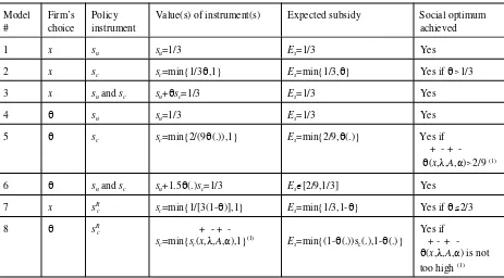
presented as a benchmark case to better situate the results that follow. Table 1 summarizes the
results of this model, as well as the models to follow, to facilitate the comparisons between the
x s A s c c ( ) ( ) ( ) = − − − α θ
γ θ θ
4 1 (11)
∂ ∂
α θ γ θ
θ γ θ
W s A s s c c c = − − − − ≥
4 1 3
4 1 0
2 2 3
3
( ) ( )
( ( ) ) (13)
sc = min{1 , }
3θ 1 (14)
[Table 1 here]
3.2 Model 2: Exogenous probability of success with conditional R&D subsidies
Now assume that the government grants only a conditional (on success) subsidy. The
expected profits of the firm become:
B(x,sc) = 2(p(yg(x))-cg(x))yg(x) + (1-2)(p(yb)-cb)yb - (1-2sc)(x2 (10)
Note that the firm gets the subsidy with probability 2. In the second stage the firm chooses R&D to
maximize (10). This yields:
Expected social welfare is given by:
W(sc) = 2 CSg(sc) + (1-2) CSb + B(sc) - 2sc(x2(sc) (12) The foc for the choice of sc is:
which yields
The optimal subsidy is declining in the probability of success. This means that riskier projects
should receive higher subsidies. This result may sound counterintuitive, but it is in line with the
objective of maximizing expected social welfare. The government aims at inducing the firm to
choose the socially optimal level of x. From (11) we see that the firm’s choice of R&D depends on
the subsidy only through the term 2sc, which represents the expected subsidy for the firm. There is
a unique level of the expected subsidy which induces the optimal choice of x by the firm. To
maintain 2sc at that optimal level, the government has to move sc in the opposite direction of the
change in 2. That is, the government has to give higher subsidies to riskier projects, and lower
subsidies to safer projects. This higher subsidy is not necessarily more costly for the government,
because the probability that the subsidy is paid is low when 2 is low.
The reason why the solution takes the form of a min function is that if 2<1/3, the formula
100% of the expenses in the case of success, but even this may be suboptimal. Social welfare would
increase if the government could cover more than 100% of R&D costs, because the higher subsidy
would increase R&D.
Taking the case 2$1/3, we can write the optimal conditional subsidy as 2sc=1/3. This form
makes it directly comparable with the optimal su given by (9). We see that in both cases the (optimal) expected subsidy, which we denote Es, is the same, Es=1/3. Therefore the objective of the
government in setting the conditional subsidy is to make the expected subsidy the same for the firm
as in the case of the unconditional subsidy. The firm is indifferent between the two policy
instruments, because it is risk neutral. For 2<1/3, however, this is not feasible, and the expected
subsidy (and therefore R&D, profits, consumer surplus, and welfare) is lower with the conditional
subsidy.
Therefore, comparing R&D levels between the two models, they will be identical for 2$1/3,
but the unconditional subsidy will yield higher levels of R&D for 2<1/3. This suggests that from a
welfare point of view, the two policy instruments are equivalent for relatively safe R&D projects,
but the unconditional subsidy is strictly superior for very risky R&D projects.
The optimal sc depends only on 2. Moreover, it is at least as large (it takes its minimal value
of 1/3 when 261) as the optimal su derived in section 3.1, to compensate for the risk associated with
conditionality.
Proposition 2. With an exogenous probability of success and conditional R&D subsidies only, the
optimal R&D subsidy is sc=min{1/32,1}, and declines with the probability of success. It induces the socially optimal level of innovation iff 2$1/3.
3.3 Model 3: Exogenous probability of success with conditional and unconditional R&D
subsidies
Consider now the more general case where the government can simultaneously use
conditional and unconditional subsidies. The expected profit of the firm becomes:
B(x,su,sc) = 2(p(yg(x))-cg(x))yg(x) + (1-2)(p(yb)-cb)yb - (1-su-2sc)(x2 (15)
profit-x s s A s s c u u c ( , ) ( ) ( ) = − − − − α θ
γ θ θ
4 1 (16)
∂ ∂
α θ γ θ
θ γ θ
∂ ∂
α θ γ θ
θ γ θ
W s
A s s
s s
W s
A s s
s s u u c u c c u c u c = − − + − − − = = − − + − − − =
4 1 3
4 1 0
4 1 3
4 1 0
2 2 2
3
2 2 3
3 ( ) ( ( )) ( ( ) ) ( ) ( ( )) ( ( ) ) (18) maximizing level of R&D is given by
Expected social welfare is given by:
W(su,sc) = 2 CSg(su,sc) + (1-2) CSb + B(su,sc) - (su+2sc)(x2(su,sc) (17) Maximizing W w.r.t. su and sc yields the following focs:
Solving for su and sc yields
su +θsc = 1
3 (19)
The solution is such that Es=1/3, the same expected subsidy as in the two previous models. There are different combinations of su and sc which can lead to the optimal outcome. Notice the substitutability of su and sc: an increase in one must necessarily lead to a decrease in the other.
Because the expected subsidy is the same as in the model with su only, all other variables
(R&D, welfare, etc.) will have the same levels. Both the firm and the government are indifferent
between the different combinations leading to the optimal expected subsidy.
However, expected welfare here is higher than in the model with sc only. Remember that in
the latter case, when 2<1/3, it is not possible to set the subsidy high enough to achieve Es=1/3; this
results in lower R&D and lower welfare. Therefore, using both su and scis superior (when 2 is low) to using sc only.
To illustrate how different combinations of conditional and unconditional subsidies can be
used to achieve the optimum, we consider three combinations. The first combination is such that sc is set as high as possible, and consequently su is set as low as possible. This combination is useful
when the government wants to rely as much as possible on conditional subsidies. The method to
however, 2<1/3, sc alone is not sufficient to attain the optimal expected subsidy; in this case we have
to set su=1-sc and substitute this equality into (19). This yields
su= − sc
− = −
1 3 3 1
2 3 1
θ
θ θ
( ), ( ) (20)
The second combination is such that su is set as high as possible, while sc is set as low as possible.
This combination is relevant when the government wants to rely mainly on unconditional subsidies.
It is easy to see from (19) that it is always possible to set sc=0 and su=1/3, achieving the optimal
expected subsidy and insulating the firm from uncertainty with respect to the subsidy to be received.
Finally, the third combination is such that su=sc=s: the government wants to set a unique level for the subsidy, with the firm getting s before the project is undertaken, and getting another time s if the project succeeds. Substituting this equality into (19) yields s=1/3(1+2).
Figure 1 shows the three types of combinations. The first combination is represented by two
curves, su min and sc max. When 2<1/3, sc is increasing in 2, while su is decreasing in 2; when
2$1/3, su=0 and sc is decreasing in 2. The second combination is simply the horizontal line su=1/3. The last combination is represented by the declining line.
[Figure 1 here]
This analysis shows the advantage of using both su and sc over using sc only. When 2$1/3, the two
approaches yield the same level of expected welfare. When, however, 2<1/3, expected welfare is
higher when both su and sc are used, because in that case it is possible to reach the optimal expected subsidy only by using a strictly positive su.
The fact that the optimal subsidy sometimes declines with 2 does not change the expected
relationship between x and 2. It is easy to verify that x always increases with 2 when su and sc are
chosen optimally.
From a policy point of view, conditional and unconditional R&D subsidies are substitutes:
they should be set such that their weighted sum is equal to 1/3; this implies that increasing one must
be parallelled by a decrease in the other.
Proposition 3. With an exogenous probability of success and both conditional and unconditional
expected subsidy is constant, and that a higher probability of success will be associated with a lower value of su and/or sc. This locus induces the socially optimal level of innovation.
4. Endogenous probability of success
We now change the focus of the model, by letting the firm choose the probability of success
of the project, rather than the extent of cost reduction. By devoting more resources to innovation,
the firm can increase the probability of success of a project leading to a cost reduction of a fixed
exogenous size, x. Let 822 represent the cost of inducing a probability of success 2. Now the subsidy
is aimed at covering part of the costs of increasing the probability of success (because x is
exogenous, its cost is irrelevant).
Note that in all three models considered until now, the functional relationship between R&D
investment and the expected subsidy is the same (equations 6, 11, and 16). This is because when the
probability of success is exogenous, all what matters for R&D investment is the expected subsidy.
As we will see, this will no longer be true when the probability of success is endogenous, because
in that case the choice of 2 will affect both the expected subsidy and the expected benefit of R&D.
4.1 Model 4: Endogenous probability of success with unconditional R&D subsidies
Consider first the case where the government uses only an unconditional subsidy. The
expected profit of the firm is:
B(2,su) = 2(p(yg)-cg)yg + (1-2)(p(yb)-cb)yb - (1-su)822 (21)
In the second stage the firm chooses 2 to maximize its expected profits, which yields
Expected social welfare is given by:
W(su) = 2(su)CSg + (1-2(su))CSb + B(su) - su822(su) (23)
In the first stage, the government chooses su to maximize (23). This yields the following foc:
Solving for the optimal unconditional subsidy we obtain
θ α
λ ( ) ( ( ) )
( )
s x A x
s u u = − + − 2
8 1 (22)
∂ ∂ α λ W s
s x A x x
s u u u = − − + − = ( )[ ( ( ) )] ( )
1 3 2
64 1 0
2 2
15
Given this solution for su, and given the solution for 2 from (23), it must be that 8>3(x(2A-")+x)/16 to get 2<1.
This constraint applies to models 5 , 6, and 8 below too.
s
x A x
c =
− +
min{
( ( ) ), } 32
27 2 1
λ
α (29)
su = 1
3 (25)
Note that this model is symmetric with respect to the model in section 3.1, where the firm chooses
x and the government chooses su, with the roles of x and 2 interchanged. Therefore, the optimal su
is the same.15
Proposition 4. With an endogenous probability of success and unconditional R&D subsidies only,
the optimal R&D subsidy is su=1/3. It induces the socially optimal level of innovation.
4.2 Model 5: Endogenous probability of success with conditional R&D subsidies
We now alter the previous model by letting the government use only conditional subsidies.
In contrast to the previous model, the symmetry with the model where the firm chooses x and the government chooses sc breaks down, because now the firm can affect not only the expected cost
reduction, but also the probability of obtaining the subsidy.
The expected profit of the firm is given by:
B(2,sc) = 2(p(yg)-cg)yg + (1-2)(p(yb)-cb)yb - (1-2sc)822 (26)
In the second stage the firm chooses 2 to maximize (26). The solution to this problem has two roots,
only one of which lies strictly between 0 and 1:
Expected social welfare is given by
W(sc) = 2(sc)CSg + (1-2(sc))CSb + B(sc) - 2(sc)sc 822(sc) (28) Maximizing (28) w.r.t. sc and solving for sc, we obtain
It is obvious that sc increases with 8 and ", and decreases with A and x. These counterintuitive
results mean that the optimal conditional subsidy is higher when the size of the innovation is lower,
θ λ λ λ α
λ
(s ) x( (A ) x s)
s
c
c
c
= 8 − 64 −48 2 − +
24 2
innovation is more costly, demand is lower and production costs are higher. These are all factors
which contribute to reducing the private and social value of the innovation.
To understand this result, we look at how the probability of success chosen by the firm varies
with the model’s parameters. Substituting the optimal conditional subsidy into 2(sc) from (29) yields
the equilibrium choice of 2:
θ α
λ
* = 3 2( ( − )+ )
16
x A x
(30)
As expected, 2 increases with A and x and declines with 8 and ". Therefore, the model parameters
affect 2 and sc in opposite directions. The effects of the parameters on 2 are intuitive. To understand
why the government reacts in the opposite direction, it is useful to calculate the expected subsidy,
Es=2*sc:
Note that (29) can be rewritten as
The optimal expected subsidy is constant. Therefore, as a change in the environment pushes 2 in one
direction, the government reacts by moving sc in the other direction, so as to maintain the expected subsidy constant. In choosing sc, the government takes into account that the choice of 2 by the firm depends on sc. Therefore, while the level of the conditional subsidy and the endogenous probability
of success depend on the model parameters, the expected subsidy does not.
In fact, the expected subsidy is lower in this model than when the firm chooses x (section
3.2) and when the firm chooses 2 while the government uses only an unconditional subsidy (section
4.1); in both cases the optimal expected subsidy was 1/3. This result has to do with the constant
optimal expected subsidy: the government uses the conditional subsidy to maintain the expected
subsidy at its optimal level.
When only sc is used, there is a risk that the government may not be able to implement the
optimal subsidy, because this would require covering more than 100% of the expenses on R&D in
θ α
λ
λ α
* ( ( ) )
( ( ) )
s x A x
x A x
c =
− +
− +
= 3 2
16
32 27 2 2
9
(31)
sc = min{2 , }
θ α λ
* = 3 2( ( − )+ )
16
x A x
(33)
case of success. From (29) it is clear that this is more likely to happen when 8 and " are high, and
A and x are low. Of particular interest is the effect of x: conditional subsidies only are less likely to
induce the socially optimal level of innovation when the size of the R&D project is small, because
a small x induces a small 2, in which case sc cannot be set high enough to induce the optimal 2.
From (32), se see that this problem occurs when 2<2/9. Therefore, if the model parameters induce
the firm to choose 2<2/9, the government will pay 100% of R&D expenditures in case of success,
but the choice of 2 by the firm will be suboptimal.
Proposition 5. With an endogenous probability of success and when the government uses only
conditional subsidies, the optimal conditional subsidy declines with the size of the innovation and demand, and increases with the cost of innovation and production costs. The optimal expected subsidy is Es=2/9. The socially optimal level of innovation is induced iff 2$2/9.
4.3 Comparison between conditional and unconditional subsidies with 2 endogenous
It is useful to compare the performance of the last two models. Comparing sc and su, we note that factors which increase sc will increase the likelihood that sc>su. Hence, a lower innovation size,
a smaller market, a higher innovation cost, and a higher production cost all increase the chances that
sc>su. It is when the conditions are particularly “unfavorable” that the conditional subsidy is likely
to be higher than the unconditional subsidy. This is in contrast to the models where the firm chooses
x (sections 3.1 and 3.2), where the conditional subsidy is always higher than the unconditional
subsidy.
We now compare the choices of 2 between the two models. Substituting the optimal su into
(22) yields the equilibrium level of 2 with unconditional subsidies:
But this is equal to the equilibrium value of 2 with conditional subsidies when sc is chosen
optimally, given by (29). Hence, the optimal subsidies are such that they induce the same choice of
the probability of success by the firm. This is not surprising: social welfare is maximized when the
firm chooses the socially optimal level of 2. Different types of subsidies should lead to the same
su + 9x 2 A− + x sc = 32
1 3 ( ( α) )
λ (37)
The equality between 2s in the two models implies that they yield identical levels of
production costs, output and expected welfare. Given that the 2s are the same, it follows that
expected production costs and output are the same. The only difference between the two models is
in terms of the expected cost of the subsidy, which is higher with unconditional subsidies, because
in this case Es=1/3, whereas it is 2/9 with conditional subsidies. But given that the subsidy is simply
a transfer from the government to the firm, its level vanishes from the welfare function. In the
presence of a positive shadow cost of public funds, however, conditional subsidies would yield a
clear advantage over unconditional subsidies.
Hence a social planner having to choose between conditional and unconditional subsidies
strictly prefers the latter when the probability of success is exogenous (and the firm chooses the size
of the innovation), but is indifferent between the two when the probability of success is endogenous
(and the size of the innovation is fixed).
4.4 Model 6: Endogenous probability of success with conditional and unconditional R&D
subsidies
Consider now the more general model where the firm chooses 2 and the government uses
su and sc. Expected profits are
B(2,su,sc) = 2(p(yg)-cg)yg + (1-2)(p(yb)-cb)yb - (1-su-2sc)822 (34)
The output stage is as above. Maximizing expected profits w.r.t. 2 yields
Expected social welfare is
W(su,sc) = 2(su,sc)CSg + (1-2(su,sc))CSb + B(su,sc) - (su+2sc)822(su,sc) (36) Maximizing social welfare w.r.t. su and sc yields
As in the model with exogenous 2 and conditional and unconditional subsidies (section 3.3), there
are different combinations which can be used to attain the optimal subsidy. To analyze this result,
θ λ λ λ
λ
( , )
( ) ( ( )) ( ( ) )
s s s s s x A R x
s u c
u u c
c =
− − − − − +
8 1 8 1 48 2
24
su + sc = 3
2
1 3
θ* (39)
we substitute the optimal subsidies into 2(su,sc) to obtain the equilibrium probability of success.
Given that all combinations satisfying (37) are socially optimal, any combination can be used for
this substitution, and will lead to the same value of 2. We choose su=0 and solve for sc from (37),
and substitute this value of sc into (35) to obtain
which is equal to the equilibrium value of 2 in the previous two models. Therefore, in all three
models with an endogenous probability of success, the goal of the government is to induce this
socially optimal choice of 2. In each case, it uses the available instrument(s) to achieve this
objective.
Note that (37) can be rewritten as
where 2* is given by (38). This way of writing the locus of optimal subsidies shows the inverse link
between R&D subsidies and the probability of success: factors which increase 2* induce the
government to reduce sc and/or su.
Note that the coefficient of sc in (39) is larger than 2, hence the r.h.s. of (39) cannot be
interpreted as an expected subsidy. To compare the expected subsidy in this model with the previous
models, we compute the expected subsidy in two extreme cases, when sc=0 and when su=0. When sc=0, it is obvious from (37) that Es=1/3, the same value as in the model with unconditional subsidies only. When su=0, the expected subsidy is
Therefore, when only sc is used, the expected subsidy is as in the previous model, where the use of su was not an option. Hence Es0[2/9,1/3]. The lower bound obtains when su=0. As su is allowed to increase, sc declines, and Es increases, until it reaches its maximum value of 1/3 when sc=0 and su=1/3.
θ α
λ
* ( ( ) )
= 3 2 − +
16
x A x
(38)
E s
x A x
x A x
s = c
The goal of the government is to induce the optimal 2. The expected subsidy is allowed to
vary to achieve this objective. As the subsidy is simply a transfer from the government to the firm,
what really matters for social welfare is the choice of the probability of success by the firm,
irrespective of how it is financed.
This illustrates one difference with the model where 2 was exogenous, where it was found
that both the expected subsidy and the choice of x were the same across all three models (except
when 2 was too low and only sc could be used). The real objective of the government there was to
induce the optimal x; the fixed expected subsidy was the appropriate instrument to achieve this
objective, because 2 was exogenous. However, with an endogenous 2, the expected subsidy may
need to vary to achieve the optimal 2.
When both su,sc>0, changes in the parameters will force the government to adjust the
subsidies. From (37), we see that increases in demand or in the size of the innovation will force the
government to reduce su and/or sc, while increases in production costs or in the cost of the innovation will induce the government to increase su and/or sc. Again, the government moves the subsidies in
a direction which is opposite to the direction in which the firm moves 2.
Proposition 6. With an endogenous probability of success and when the government can use both
conditional and unconditional subsidies, the government chooses a mixture of su and sc based on (37) to induce the firm to choose the optimal 2 given by (38). The optimal subsidies decline with demand and the size of the innovation, and increase with production costs and innovation costs. The expected subsidy Es, [2/9,1/3]. The socially optimal level of innovation is induced.
5. Reverse conditional R&D subsidies
In some cases the firm gets the subsidy only if the project fails. For instance, if the project
succeeds and the firm generates revenues from the commercialization of its products, the firm has
to pay the government part or all of the subsidy it received. We consider this type of subsidy when
the firm chooses x, and then when it chooses 2.
5.1 Model 7: Exogenous probability of success with reverse conditional R&D subsidies
x s A s c R c R ( ) ( ) ( ( ) ) = − − − − α θ
γ θ θ
4 1 1 (42)
∂ ∂
α γ θ θ θ θ
θ γ θ
W s A s s c R c R c R = − − − − − − − ≥
4 1 3 1 1
4 1 1 0
2 2 2
3
( ) ( ( )) ( )
( ( ( )) ) (44)
scR =
−
min{
( ), } 1
3 1 θ 1 (45)
with a reverse conditional subsidy, the firm gets the subsidy only if the project fails, which occurs
with probability 1-2. Let sRc denote this reverse conditional subsidy. The expected profits of the firm
are:
B(x,sRc) = 2(p(yg(x))-cg(x))yg(x) + (1-2)(p(yb)-cb)yb - (1-(1-2)sRc)(x2 (41)
The choice of output is unchanged. In the second stage the firm chooses R&D, which yields
Expected social welfare is given by:
W(sRc) = 2 CSg + (1-2) CSb + B(sRc) - (1-2)sRc(x2(sRc) (43) The foc for the choice of sRc is:
Solving for sc yields
Notice that now the optimal conditional subsidy is increasing in 2. Hence safer R&D projects should
receive higher subsidies. Remember that the goal of the government is to induce the optimal choice
of x. When 2 is low, the probability that the firm will have to repay the subsidy is low; hence a small subsidy is sufficient to induce the firm to choose the optimal x. When 2 is high, however, there are
good chances that the subsidy will have to be repaid. To compensate for that, the subsidy has to be
large enough. Hence the incentive effects of the subsidy when it is based on failure are opposite to
those obtained when the subsidy was conditional on success.
From (45) we see that when 2$2/3 the government sets sRc=1. When 2 is very high, the
government would like to set the subsidy at a very high level to compensate for the fact that the firm
will very likely have to pay it back; in fact the government would like to set sc>1. But as this is not allowed, the government settles for sRc=1. This means that for this range of 2, the subsidy is
suboptimal, and induces a suboptimal R&D effort. Again, because 2 increases with x, this effect is
more likely to obtain when the innovation is important.
When sRc takes its optimal value, Es=(1-2)sRc=(1-2)/[3(1-2)]=1/3. This is the same expected
16
Figure 3 is based on the numerical parametrization A=1000, "=50, (=60.
π π α γ θ θ
γ θ γ θ θ θ
R SUC A for
− = − − −
− − − > ∈
( ) ( )
( )( ( ) ) ( , )
2 2 2
1 3
1 3
8 3 4 1 0 0 (46)
expected subsidy is required to induce the optimal R&D investment.
To compare sc with sRc, figures 2 and 3 illustrate the equilibrium subsidies and R&D outputs
under the two subsidy schemes.16 The two subsidies are equal when 2=0.5. For lower values of 2,
the subsidy based on success is higher, while the opposite is true for higher values of 2. As for R&D,
the two subsidy schemes yield exactly the same R&D effort when 20[1/3,2/3]. When 2<1/3, the
subsidy based on failure yields a slightly higher R&D effort. This is due to the fact that in this range
the subsidy based on success, even though it is higher, is suboptimal. When 2>2/3, the subsidy based
on success yields significantly higher R&D effort. This is because in this range the subsidy based
on failure is suboptimal. While figure 3 may suggest that in this range R&D is constant when the
subsidy is based on failure, in fact it is slightly increasing. In this range R&D is very flat because
the subsidy is stagnating while 2 is increasing, which results in a reduction in the expected subsidy;
this dampens the incentives for R&D considerably.
[Figures 2 and 3 here]
As figure 3 shows, the gap in R&D due to the suboptimality of the subsidy based on success when
2 is low is marginal, while the gap in R&D due to the suboptimality of the subsidy based on failure
when 2 is high is significant. This suggests that it is less costly to have a suboptimal R&D subsidy
when the probability of success is low, in which case R&D is low anyway, than when the probability
of success is high, in which case R&D is higher and is more socially valuable.
Comparing expected profits between the two conditional subsidy schemes, it is easy to see
that the firm loses from the suboptimality of the subsidy. Consider the range 20[0,1/3]. Let BR
represent profits with the reverse subsidy, and BSUC represent profits with the subsidy conditional
on success. In this range, sc=1, while sRc=1/3(1-2). Substituting into the profit functions and taking
the difference yields
In this range the subsidy based on success is suboptimal, while the subsidy based on failure is
optimal, hence expected profits are higher with the latter subsidy.
π π α γ θ
γ θ γ θ θ
R SUC A for
− = − − −
− − < ∈
4 2 3
3 8 3 4 0 1
2 2 2
2 2
2 3
( ) ( )
( )( ) ( , ] (47)
functions and taking the difference yields
In this range the subsidy based on success is optimal, while the subsidy based on failure is
suboptimal, hence expected profits are higher with the subsidy based on success.
The welfare comparison goes in the same direction as the comparison of R&D and profits.
Hence, for risky R&D projects, a subsidy which is paid to the firm only in the case of failure is
preferred. For safe R&D projects, a subsidy paid in the case of success is superior. For intermediate
levels of risk, the two subsidy schemes are equivalent. It is important to remember that here we
compare only the two conditional subsidy schemes, and do not take into account other schemes
which make use of unconditional subsidies (exclusively, or in conjunction with conditional
subsidies), which easily resolve this suboptimality problem.
Proposition 7. When the probability of success is exogenous and the government uses a reverse
subsidy scheme such that the subsidy is paid only when the R&D project fails, the optimal subsidy is given by (45) and increases with the probability of success. The socially optimal level of innovation is induced iff 2#1/3.
Proposition 8.With an exogenous probability of success, comparing only conditional subsidies, the
subsidy based on failure generates more R&D and welfare in the range 20[0,1/3], and generates less R&D and welfare in the range 20[2/3,1]. The two subsidy schemes are equivalent for intermediate levels of risk.
5.2 Model 8: Endogenous probability of success with reverse conditional R&D subsidies
It is useful to consider the use of reverse subsidies when the firm chooses the probability of
success. On the one hand, this will allow us to compare regular conditional subsidies (from section
4.2) with reverse conditional subsidies with 2 endogenous. On the other hand, this will establish
whether the comparison between regular conditional subsidies and reverse conditional subsidies
performed above is robust to the choice variable of the firm.
expected profits of the firm are:
B(2,sRc) = 2(p(yg)-cg)yg + (1-2)(p(yb)-cb)yb - (1-(1-2)sRc)822 (48)
Optimal output is as above. The expected profit-maximizing choice of 2 is
Expected welfare is given by:
W(sRc
) = 2(sRc)CSg + (1-2(sRc))CSb + B(sRc) - 2(sRc)sRc822(sRc) (50)
Maximizing (50) w.r.t. sRc yields
The reverse conditional subsidy increases with A and x, and decreases with " and 8. This is in
contrast to model 5, where the conditional subsidy varied in opposite directions with the model
parameters. The reason for that differential lies in the effect of the change in firm behavior on the
expected subsidy. In both models there is an optimal expected subsidy, which is required to induce
the firm to choose the optimal 2. Consider, for example, the effect of an increase in x on 2 and on
the conditional subsidy. In both models (5 and 8), an increase in x increases the socially optimal
level of 2, and also the 2 chosen by the firm. However, remember that the firm will choose the
socially optimal 2 iff it receives the optimal expected subsidy. In model 5, the increase in 2 by the
firm increases the expected subsidy, which is given by 2sc. Therefore, to maintain the expected
subsidy at its optimal level, the social planner moves sc in the opposite direction. In model 8,
however, when the firm increases 2 in response to an increase in x, it reduces the probability of
obtaining the subsidy, because the subsidy is obtained only if the project fails. Therefore Es=(1-2)sRc
is reduced; to maintain the optimal level of 2, the government has to increase Es, and the only way
to do this is to increase sRc. The effects of changes in A, ", and 8 can be understood in the same
manner.
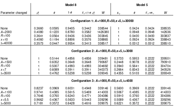
Given the relative analytical complexity of (49) and (51), the behavior of innovation and
subsidies in this model is best analyzed using numerical simulations. This is done in table 2. The left
part of table 2 illustrates the optimal reverse conditional subsidy, the choice of 2 by the firm, the
probability of obtaining the subsidy (1-2), the expected subsidy, and total welfare for different
parameter configurations. Three sets of benchmark configurations are considered, and for each
θ λ α λ λ
λ
(s ) x( (A ) x s) ( ( s )) ( s )
s c R c R c R c R c R
= 12 2 − + + 2 1− − 4 1−
12
2
(49)
s
x A x
c R = − − + min{ ( ( ( ) )), } 32
3 32 9 2 1
λ
benchmark configuration each parameter is varied.
[Table 2 here]
First note that 2 increases with x and A, and declines with " and 8. This is intuitive, and in
accordance with the comparative statics derived above for both x and 2.
One difference between models 5 and 8 is that in model 5, at an interior solution, the optimal
expected subsidy is fixed at Es=2/9. In model 8, however, even at an interior solution, the optimal
expected subsidy is not constant, but varies with the model parameters. Moreover, the optimal
expected subsidy at an interior solution varies in the same direction as 2 and sc: it increases with A
and x, and declines with " and 8.
Consider now the three configurations in the left part of table 2. The main difference between
these configurations, beyond the specific numerical values used, is that in the first and third
configurations, the solution is interior, and the subsidy, expected subsidy, and 2 are all socially
optimal. In the second configuration, however, welfare is increasing in sRc at sRc=1, hence the optimal subsidy is sRc=1. In this case the subsidy is suboptimal, and so is the choice of 2 by the firm. Note
that the second configuration obtains for 8=3000, which is lower than the value of 8 used for the
first and third configurations. This is consistent with the comparative statics described above, where
the optimal sRc decreases with 8. As 8 becomes very low, sRc reaches its maximum of 1, and the subsidy becomes suboptimal. Because x has the opposite effect of 8 on 2 and sRc, it can also be said that the reverse subsidy is more likely to be suboptimal when x is high.
One difference between the interior and corner solutions is that in the first and third
configurations (interior solutions), Es increases following any change which increases sRc
. This means
that the increase in sRc is larger than the decrease in 1-2, which increases Es. In the second configuration, however, we have a corner solution, and Es declines when x or A increase, for instance. This is because sRc is already set at its maximum value; hence any change which increases
2 reduces the expected subsidy.
It is also obvious from the table that welfare moves in the same direction as sRc, the expected
subsidy (at an interior solution), and 2. Therefore, a change in the environment which increases
5.3 Comparison between conditional and reverse conditional subsidies when the probability
of success is endogenous
One relevant question is whether conditional subsidies awarded in the case of success (model
5) are preferred to conditional subsidies awarded in the case of failure (model 8). This comparison
was already established between models 2 and 7, where the choice variable of the firm was x. Here
we wish to answer this question in the context of 2 as a choice variable.
The right side of table 2 illustrates the optimal subsidy, the choice of 2 by the firm, the
expected subsidy, as well as welfare from model 5, where the regular conditional subsidy was used.
These values come from the solutions given by (29) and (30). The same numerical parametrization
is used as for model 8 to facilitate the comparison.
The three configurations allow us to establish a complete comparison between the two
models, because each model can have either an interior or a corner solution for the choice of subsidy
by the government. In configuration 1, model 8 is at an interior solution, while model 5 is at a corner
solution. In the second configuration, model 5 is at an interior solution, while model 8 is at a corner
solution. Finally, in the third configuration, both models are at interior solutions. The structure and
the results of model 5 have been discussed above, here the focus is on the comparison of the two
models. The easiest way to compare them is to read table 2 horizontally; that is, for given parameter
values, to compare the subsidy level, the choice of 2, the expected subsidy, and social welfare.
In configuration 1, sRc is optimal, while sc is suboptimal. This results in a situation where EsR>Es, WR>W and 2R=2W>2, where 2W denotes the socially optimal level of 2. Hence, in this case,
the reverse conditional subsidy is preferred to the (success based) conditional subsidy. Because the
parameter values are such that the equilibrium and optimal choices of 2 are rather low, this makes
it impossible (in model 5) to set sc high enough to achieve the optimal expected subsidy, which is
fixed.
In configuration 2, exactly the opposite occurs. sc is optimal, while sRc is suboptimal. It
follows that 2=2W>2R and W>WR. And this is true even though EsR>Es. But because the endogenous
probability of success is lower with the reverse subsidy, welfare is lower. In this case the equilibrium
choices of 2 are quite high; this reduces the probability of obtaining the subsidy in the reverse
subsidy model, forcing the government to raise sRc to its maximum.
results in lower welfare. This is because even a subsidy of 100% may be suboptimal if it does not
induce the efficient level of effort by the firm. In that case, such a high subsidy is an indication that
the government would like to set the subsidy at an even higher level to achieve the optimum, but is
unable to. Whereas when the subsidy is strictly below 1, the constraint is not binding.
Finally, in configuration 3, the two models yield identical levels of 2 and W. Both models
are at an interior solution, and both are equivalent. But this identical outcome is achieved differently.
In this case the choice of 2 is intermediate. This allows the government to achieve the optimal 2 by
setting a reverse conditional subsidy which is quite high, but lower than 1. At the same time, it
allows the government to achieve the optimal 2 in model 5. Note that for this configuration sRc>sc:
a higher reverse conditional subsidy is required.
This comparison between regular conditional subsidies and reverse conditional subsidies
with 2 endogenous yields results which are of the same spirit as those obtained from the comparison
of models 2 and 7, where x was the choice variable. There it was found that for low (exogenous)
values of 2, the reverse conditional subsidy is preferred; for high values of 2, the regular conditional
subsidy is preferred; and for intermediate values of 2, the two models are equivalent. The
comparison performed in the current section between models 5 and 8 goes in the same direction, and
shows that this intuition extends to the case where 2 is endogenous.
Proposition 9. When the probability of success is endogenous and the government uses a reverse
subsidy scheme such that the subsidy is paid only when the R&D project fails, the optimal subsidy increases with the size of the project and demand, and declines with production costs and innovation costs. The socially optimal level of innovation is induced iff the probability of success chosen by the firm is sufficiently small.
Proposition 10.With an endogenous probability of success, comparing only conditional subsidies,
6. Conclusions
This paper has analyzed how R&D subsidies can be made conditional on the success or
failure of R&D projects, and how these conditional subsidies can be used on a stand-alone basis, or
in conjunction with more traditional unconditional subsidies.
In general, the model warns against the use of conditional R&D subsidies alone. For a wide
range of project sizes and degrees of riskiness, conditional subsidies alone may yield suboptimal
levels of innovation. This problem can be avoided by combining conditional and unconditional R&D
subsidies to achieve the optimal expected subsidy. In some cases, conditional subsidies yield a lower
expected cost of the subsidy to the government. As for the choice between conditional subsidies
based on success and those based on failure, the former are preferred for safer R&D projects, while
the latter are superior for risky R&D projects.
The result that the optimal conditional subsidy varies negatively with the probability of
success sheds light on the debate of when R&D subsidies contribute to increasing R&D, and when
they finance research activities firm would undertake anyway. The argument that the subsidy should
be positively correlated with the social profitability from innovation (size of innovation, market size,
probability of success, etc.) overlooks the fact that many of the factors which increase the social
value of the innovation also increase its private value to the innovator, increasing the privately
optimal investment. Hence, the innovator already accounts for a large number of these factors, and
it may be redundant for the government to subsidize R&D projects because they are promising or
socially beneficial; the innovator’s actions already reflect partly those benefits. Rather, it is when
the private value of the innovation is small (due to a small market size, a low probability of success,
etc.) that government intervention is most needed.
Tassey (1996) cites evidence from surveys by the Industrial Research Institute and others,
which “show a definite decline in recent years in industry’s willingness to fund longer-term,
higher-risk technology research” (p. 581). R&D subsidies which reward success can contribute to
alleviating this particular market failure. Alternatively, to provide more safety for firms, a reverse
conditional subsidy could be used, which results in a high probability that the firm keeps the
subsidy, given the high probability of failure.
In the current model the problem of overinvestment in R&D has not arisen. This is due to