Interregiona;Decomposition of labor productivity differences in China, 1987 1997

Munich Personal RePEc Archive

Interregiona;Decomposition of labor

productivity differences in China,

1987-1997

Yang, Ling and Lahr, Michael/L

Rutgers, The State University of New Jersey

4 April 2008

Online at

https://mpra.ub.uni-muenchen.de/8313/

INTERREGIONAL DECOMPOSITION OF

LABOR PRODUCTIVITY DIFFERENCES IN CHINA, 1987-1997

Ling Yang

School of Economics and Finance, Xi’an Jiaotong University, Xi’an 710061, China. E-mail: [email protected]

Michael L. Lahr

Center for Urban Policy Research, Rutgers, The State University of New Jersey, New Brunswick, NJ, 08901-1982. E-mail: [email protected]

ABSTRACT: The literature on regional disparities in China is both broad and deep.

Nonetheless much of its focus has been on the effects of trade liberalization and national policies toward investment in interior provinces. Few pieces have examined whether the disparities might simply be due to differences in industry mix, final demand, or even interregional trade. Using multiregional input-output tables and disaggregated

employment data, we decompose change in labor productivity growth for seven regions of China between 1987 and 1997 into five partial effects—changes in value added

coefficients, direct labor requirements, aggregate production mix, interregional trade, and final demand. Subsequently we summarize the contributions to labor productivity of the different factors at the regional level. In this way, we present a new perspective for recent causes of China’s interregional disparity in GDP per wroker.

Keywords: Decomposition, input-output analysis, productivity, regional disparity, China

1. INTRODUCTION

As GDP has soared, interregional income disparity has become a major policy

challenge in China due to increasing concerns about social stability (Démurger, 2001).

From 1952 to 2006, China’s GDP grew at an annual average rate of 7.9 percent and even

more rapidly during the last three decades—9.6 percent annually from 1978 to 2006. The

share of GDP produced by provinces in coastal China, its central part, and its extreme

west over the same period reveals some growth imbalance. While the coastal provinces

produced 48.6 percent of GDP in 1952, their share increased to 65.8 percent by 2006.

Most of the coast’s gains in share were at the expense of central and western China,

whose shares of GDP, respectively, dropped from 32.8 percent and 18.6 percent in 1952

to 21.7 percent and 12.5 percent in 2005.1

Some of the regional shifts were induced by national economic reforms

implemented since 1978. Preferential policies for the coastal provinces were a key initial

element of the reformation programs designed to jump start world trade. During the

1980s, Shenzhen, Zhuhai, Shantou, Xiamen cities and Hainan province were designated

special economic zones and Dalian, Guangzhou, Shanghai etc altogether14 more cities

were designated open coastal cities. Preferential policies were given in tax, projects and

foreign exchange to attract foreign investment and business and these places have

become a window of China’s opening to the outside world and regarded as “growth pole”

for the economy of whole China. Whether or not these policies actually caused the

subsequent growth remains unclear, but particularly strong growth ensued in the coastal

economies nonetheless. Of course, this growth also exacerbated pre-existing regional

income disparities. In response to the deepening interregional income disparities, China’s

national government proposed the development strategy for different regions in China

based on their history and situation. China proposed West Development Strategy in 1999,

the polices in the West is mainly for increasing the capital input, improving the

investment environment such as infrastructure, deepening the reform and opening,

1

strengthening the supporting of technology, education and human resource. In 2002,

China proposed Revitalization of the Traditional Industrial Bases in Northeast China,

more emphasis is laid on institutional innovation, with the restructuring of state-owned

enterprises, upgrading industry structure and promoting modern tertiary industry, creating

jobs for the unemployed and providing social security, promoting sustainable

development of resource-based cities, developing modern agriculture and so on. In 2004

Central China Rising was proposed, the policies for traditional industrial bases will be

according to those in Northeast and other underdeveloped places according to polices in

West of China. The policies are supposed to help promote establishment of grain

production base, energy’s raw material base, modern equipment manufacturing base and

hi-tech industry base in Central China.

Literature investigating the causes of interregional disparity in China has cited

specific likely causes of the increasing differences in per capita GDP across regions.

Some factors that have been tested are differences in the infrastructure development like

the network of transportation and telecommunication (Démurger 2001), the source, size

and sectoral allocation of fixed investment (Wei 2000), the speed in the adoption of new

technology, level of human capital stock (Liu and Li 2006), the accessibility to foreign

direct investment and international trade (Sun and Parikh, 2001, Wei and Wu, 2001), the

labor market distortions in particular Hukou system impedes labor mobility from rural to

urban (Cai et al. 2002), and province-specific public policy strategies (Yang, 2002, Lin

and Liu, 2005, Kanbur and Zhang, 2005, Démurger et al., 2002a,b).

Most of the research cited in the last paragraph adopts a neo-classical economic

growth approach applying the hypothesis that productivity is converging across the

regions analyzed. Few pieces have examined whether the disparities and any convergence

across them might simply be due to differences and changes in industry mix, in

interregional trade, or even in the composition of final demand. Li and Haynes (2008) use

shift-share method to analyze China’s regional disparity at province level from an

industry structure point of view. The fact that China’s industries are interdependent as

expressed in input-output (I-O) parlance has nearly been completely overlooked. Keidel

not been so much led by a surge in exports but instead by fluctuations in domestic

demand.

We take a different tack in our analysis of Chinese interregional productivity; we

use the country’s 1987 and 1997 multiregional input-output (MRIO) tables with seven

regions, disaggregated employment data, and a decomposition approach introduced by

Dietzenbacher et al. (2000). This approach decomposes productivity into five partial

effects—changes in value added coefficients, direct labor requirements, aggregate

production mix, technology change, interregional trade and final demand.2 Subsequently

we summarize the contributions to labor productivity of the different factors at the

regional level.

The paper is organized as follows. Section 2 outlines our research approach.

Section 3 is a general description of data used in this paper. In Section 4, we analyze the

results of our decomposition. A final section concludes the paper.

2. RESEARCH APPROACH

There are many ways to examine the likely causes of productivity change. We are

particularly interested to learn the multifarious guises China’s economic reforms sported

in affecting interregional income disparity. Was technological change a major player?

How about changes in interregional trade? Perhaps the disparity was enhanced by the

degree to which different sectors managed to discover ways outside of technological

change to save on labor costs. How much did margin reducing pressures of international

trade affect per capita GDP across regions? Were most of the disparities introduced via

manufacturing, which is what is largely traded, or did other sectors play a role? After

considering the sorts of issues we were interested in answering, it became that the

multiplicative decomposition method introduced by Dietzenbacher et al. (2000) was best.

The following presents Dietzenbacher et al.’s approach, as we adopted it. Let N be

the number of industries in each region and C be the number of regions. The other

definitions are as follows:

v: aggregate value added (scalar);

2

l: aggregate labor inputs (scalar);

π: aggregate labor productivity (v/l) (scalar);

A: matrix with input coefficients (NC×NC matrix), with typical element denoting the

input of product i from region r per unit of output in industry j in region s;

rs ij

α

L: Leontief-inverse (NC×NC matrix), L≡(I-A)-1;

x: vector with χir denotes the gross output level of industry i in region r (NC×1 vector);

f: vector with element denotes the final demand for output of industry i in region r

(NC×1 vector);

r i

f

λ: vector with elements giving the use of labor per unit of gross output in industry i in

region r (NC×1 vector);

r i

λ

μ: vector with elements giving the value added per unit of gross output in industry i

in region r (NC×1 vector);

r i

μ

A*: matrix constructed by stacking C identical N×NC matrices of aggregate intermediate

inputs per unit of gross output by industry by region (NC×NC matrix),

;

[ ]

_∑

: α α

A

T : matrix of intermediate trade coefficients, representing the shares of each region in

aggregate inputs, by input by industry by country (NC×NC

matrix), rs rs ij rs ij ij t α α∗ ⎡ ⎤ = ⎣ ⎦ _{⎡ ⎤} ⎣ ⎦ A

, note that rs 1

r⎡ ⎤ =⎣ ⎦t ij

∑

;

It follows that

v=μ'x and l=λ'x

x=Ax+f=(I-A)-1f=Lf,

and, thus

v=μ'Lf and l=λ'Lf

in which primes indicating transposed vectors. The aggregate labor productivity change

can be written as:

' '

0

1 1 1 1 1 1 1 1

' '

0 0 1 0 1 1 0 0

l v v l

π

π = × = × 0

μL f λL f

=

' 1 1 1 ' 0 1 1

⎛ ⎞

⎜ ⎟

⎝ ⎠

μL f

μ L f

' 0 1 1 ' 1 1 1

⎛ ⎞

⎜ ⎟

⎝ ⎠

λ L f

λ L f

' '

0 1 1 0 0 1

' '

0 0 1 0 1 1

⎛ ⎞

×

⎜ ⎟

⎝ ⎠

μ L f λ L f

μ L f λ L f

' '

0 0 1 0 0 0

' '

0 0 0 0 0 1

⎛ ⎞

⎜ ⎟

⎝ ⎠

μ L f λ L f ×

μ L f λ L f

By using L= (I-A* ◦TA)-1(◦ represents elementwise multiplication), we can get the final

decomposition of labor productivity change:

(1) =

0 1

π π

(1.1)×(1.2) × (1.3) × (1.4) × (1.5)

with

(1.1)=

' 1 1 1 ' 0 1 1

⎛ ⎞

⎜ ⎟

⎝ ⎠

μ L f

μ L f

(1.2)=

' 0 1 1 ' 1 1 1

⎛ ⎞

⎜ ⎟

⎝ ⎠

λ L f

λL f

(1.3)=

(

)

(

)

(

)

(

)

' * ' *

0 1 1 0 0 1

' * ' *

0 0 1 0 1 1

⎧ _{⎡ ⎤ ⎡ ⎤} ⎫ ⎪ ⎣ ⎦ _× ⎣ ⎦ ⎪ ⎨ ⎬ ⎡ ⎤ ⎡ ⎤ ⎪ _{⎣ ⎦ ⎣ ⎦} ⎪ ⎩ ⎭ -1 -1 Α Α 1 -1 -1 Α Α 1

μ Ι- Α Τ f λ Ι- Α Τ f

μ Ι- Α Τ f λ Ι- Α Τ f

D D

D D

1

1

(1.4)=

(

)

(

)

(

)

(

)

-1 -1

' * *

0 0 1 1 0 0

-1 -1

' * *

0 0 0 1 0 1

⎧ _{⎡ ⎤ ⎡ ⎤} ⎫ ⎪ ⎣ ⎦ ⎣ ⎦ ⎪ ⎨ ⎬ ⎡ ⎤ ⎡ ⎤ ⎪ _{⎣ ⎦ ⎣ ⎦} ⎪ ⎩ ⎭

Α ' Α

0

Α ' Α

0

μ Ι- Α Τ f λ Ι- Α Τ f

×

μ Ι- Α Τ f λ Ι- Α Τ f

D D D D 1 1 (1.5)= ' '

0 0 1 0 0 0

' '

0 0 0 0 0 1

⎛ ⎞

⎜ ⎟

⎝ ⎠

μ L f λ L f ×

μ L f λ L f

in which indices are time indicators, 0 denoting 1987 and 1 denoting 1997..

Equation (1.1) represents the productivity effects of changes in the value added

figures per unit of gross output by industry; Equation (1.2) represents the effects of

changed labor requirement per unit of gross output by industry; Equation (1.3) represents

the effects pf changes in the interindustry structure (due to technological change, factor

substitution, changing output compositions within industries, etc. ); Equation (1.4) is the

productivity effects of changed structures with respect to commodities and services used

as intermediate inputs; Equation (1.5) is the effects of changes in the final demand.

There is an obvious index-number problem here, so the other polar decomposition

is expressed as follows:

(2) =

0 1

π π

with

(2.1)=

' 1 0 0 ' 0 0 0

⎛ ⎞

⎜ ⎟

⎝ ⎠

μL f

μ L f

(2.2)=

' 0 0 0 ' 1 0 0

⎛ ⎞

⎜ ⎟

⎝ ⎠

λ L f

λL f

(2.3)=

(

)

(

)

(

)

(

)

-1 -1

' * *

1 1 0 0 0

-1 -1

' * *

1 0 0 0 0 0

⎧ _{⎡ ⎤ ⎡ ⎤} ⎫ ⎪ _{⎣ ⎦ ⎣ ⎦} ⎪ ⎨ ⎬ ⎡ ⎤ ⎡ ⎤ ⎪ _{⎣ ⎦ ⎣ ⎦} ⎪ ⎩ ⎭

Α ' Α

0 1

Α ' Α

1

μ Ι- Α Τ f λ Ι- Α Τ f

×

μ Ι- Α Τ f λ Ι- Α Τ f

D D

D D

0

0

(2.4)=

(

)

(

)

(

)

(

)

' * ' *

1 1 1 0 1 1 0

' * ' *

1 1 0 1 1 1 1

⎧ _{⎡ ⎤ ⎡ ⎤} ⎫ ⎪ _{⎣ ⎦ ⎣ ⎦} ⎪ ⎨ ⎬ ⎡ ⎤ ⎡ ⎤ ⎪ _{⎣ ⎦ ⎣ ⎦} ⎪ ⎩ ⎭ -1 -1 Α Α -1 -1 Α Α

μ Ι- Α Τ f λ Ι- Α Τ f

×

μ Ι- Α Τ f λ Ι- Α Τ f

D D D D 0 0 (2.5)= ' '

1 1 0 1 1 1

' '

1 1 0 1 1 1

⎛ ⎞

⎜ ⎟

⎝ ⎠

λL f

μL f ×

μL f λ L f

When we decompose for each region and industry, we replace the vectors and in

Equations (1) and (2) by diagonal matrices with the same elements on the main diagonal

and zeroes elsewhere, and premultiply all numerators and denominators with (1×NC)

aggregation vectors, one for each region or industry.

λ μ

3. DATA

The data used in our paper are multiregional input-output (MRIO) tables of China

in 1987 (Ichimura and Wang, 2003) and 1997 (China’s State Information Center [SIC],

2005). The two MRIO tables unfortunately are not perfectly consistent. The main source

of data for the 1987 MRIO is a set of 30 regional I-O tables produced by various

provinces, autonomous regions, and municipalities of China. The MRIO table for 1997

was produced using hybrid techniques with interregional trade flows based on survey

data.3 We were forced to undertake some procedures to make them comparable.

3

Prior to the present paper, others have used these two sets of MRIO tables. Meng

and Qu (2007) have used them to decompose gross output growth, rather than labor

productivity change. They focused upon the nature of interregional relationships,

however. They highlighted the performance of China’s industrial and regional

development policies on the magnitudes of interregional spillovers and feedbacks, which

is a rather different focus from that we present here. Hioki and Okamoto (forthcoming)

also the same tables, but they applied a qualitative input-output approach to identify

changes in the largest spatial linkages among China’s main regions since undertaking

reforms. In sum, while the two tables have some compatibility problems, there two

research groups showed that the worst of them can be overcome in a satisfactory manner.

To make some limitations to our study clear, we start by explaining how we dealt

with differences in region definitions across the two MRIO tables. There were altogether

seven regions in 1987 and eight in 1997. Thus, in the 1997 accounts we aggregated the

North Municipalities with North Coast, the result of which conformed with the North

China region in the geography of the 1987 MRIO accounts (see Table 1 for details).

Another change between 1987 and 1997 in Chinese political geography was that in 1987

Chongqing was included within Sichuan province, while in 1997 it was a separate

municipality directly under the central government. Fortunately within the I-O accounts

this was not an issue since both are assigned to the Southwest region in both years. But a

discrepancy does arise in the assignment of Inner Mongolia to regions in the MRIO

accounts: it belongs to North China in 1987 but to the Northwest in 1997. Unfortunately,

we have no way to correct for this problem since more detailed region classifications are

lacking. We proceeded as if this was not an issue. Since Inner Mongolia is economically

rather small.4 Of course, there was the prospect that it could produce some bias in our

results.

As for the sector classification, there were 9 industries in 1987 MRIO table and

17 in 1997 MRIO table. We also faced the additional constraint of needing employment

counts in order to measure labor productivity by industry and region in both 1987 and

4

1997. Unfortunately, we could only get labor data for five more aggregated industries by

region over the period of study. Table 2 compares characteristics of the 1987 and 1997

MRIO tables and for the employment data we used for the two years. Note, that beyond

labor data issues some other industry-based accounting issues could not be avoided. The

postal and telecommunication industry are in the Service sector in 1997 table but in Trade

and Transportation sector in 1987; eating and drinking establishments are included in the

Service sector in 1997 table but in Trade and Transportation sector in 1987 table.

Referring to the construction of the trade coefficient matrices TA, we assign the

trade coefficient to be zero when the use of an industry’s output by an industry is zero;

we assign the same value as the corresponding trade coefficient for the other year when

the total use was zero in one year but positive in the other. This implies in these situations

that all labor productivity will be attributed to changes in the input structure and none to

Table 1. China MRIO Region Definitions, 1987 and 1997

1987 1997 Region

(Abbreviation)

Provinces Region (Abbreviation)

Provinces

North East (NE) Liaoning, Jilin, Heilongjiang

Northeast (NE) Liaoning, Jilin, Heilongjiang

North China (NC) Beijing, Tianjin Hebei, Shandong

Inner Mongolia

North Municipalities North Coast

(NC)

Beijing, Tianjin Hebei, Shandong

East China (EC) Shanghai, Jiangsu, Zhejiang East China (EC) Shanghai, Jiangsu, Zhejiang South China (SC) Guangdong, Fujian, Hainan South Coast (SC) Guangdong, Fujian, Hainan Central China (CC) Shanxi, Henan, Anhui

Hubei, Hunan, Jiangxi

Central China (CC) Shanxi, Henan, Anhui Hubei, Hunan, Jiangxi North West (NW) Shaanxi, Gansu, Ningxia

Qinghai, Xinjiang

Northwest (NW) Shaanxi, Gansu, Ningxia Qinghai, Xinjiang

Inner Mongolia

South West (SW) Sichuan, Guizhou, Yunnan Guangxi, Tibet

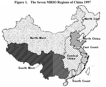
Southwest (SW) Sichuan,Chongqing, Guizhou, Yunnan, Guangxi, Tibet

Figure 1. The Seven MRIO Regions of China 1997

Source: Hioki and Okamoto (forthcoming)

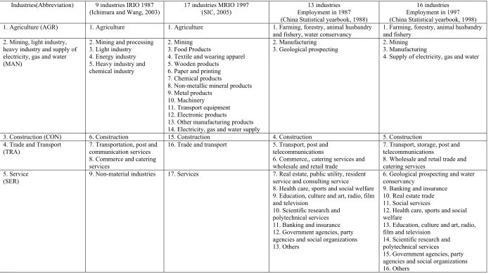
Table 2. Comparison of industries for MRIO1987 and MRIO 1997 and employment data

Industries(Abbreviation) 9 industries IRIO 1987 (Ichimura and Wang, 2003)

17 industries MRIO 1997 (SIC, 2005)

13 industries Employment in 1987 (China Statistical yearbook, 1988)

16 industries Employment in 1997 (China Statistical yearbook, 1998) 1. Agriculture (AGR) 1. Agriculture 1. Agriculture 1. Farming, forestry, animal husbandry

and fishery, water conservancy

1. Farming, forestry, animal husbandry and fishery

2. Mining, light industry, heavy industry and supply of electricity, gas and water (MAN)

2. Mining and processing 3. Light industry 4. Energy industry 5. Heavy industry and chemical industry

2. Mining 3. Food Products

4. Textile and wearing apparel 5. Wooden products

6. Paper and printing 7. Chemical products

8. Non-metallic mineral products 9. Metal products

10. Machinery

11. Transport equipment 12. Electronic products

13. Other manufacturing products 14. Electricity, gas and water supply

2. Manufacturing 3. Geological prospecting

2. Mining 3. Manufacturing

4. Supply of electricity, gas and water

3. Construction (CON) 6. Construction 15. Construction 4. Construction 5. Construction

4. Trade and Transport (TRA)

7. Transportation, post and communication services 8. Commerce and catering services

16. Trade and transport 5. Transport, post and telecommunications

6. Commerce,, catering services and wholesale and retail trade

7. Transport, storage, post and telecommunications

8. Wholesale and retail trade and catering services

5. Service (SER)

9. Non-material industries 17. Services 7. Real estate, public utility, resident service and consulting service

8. Health care, sports and social welfare 9. Education, culture and art, radio, film and television

10. Scientific research and polytechnical services 11. Banking and insurance 12. Government agencies, party agencies and social organizations 13. Others

6. Geological prospecting and water conservancy

9. Banking and insurance 10. Real estate trade 11. Social services

12. Health care, sports and social welfare

13. Education, culture and art, radio, film and television

14. Scientific research and polytechnical services

Since I-O tables are in value terms and both MRIO tables are in nominal prices,

we had to either deflate the values in the 1987 table or deflate those in the 1997 to

eliminate price effects. We opted to deflate the 1997 input-output table to make its values

consistent with those in 1987. This also enabled us to preserve information from the

original data, because there are 17 industries in 1997 and 9 industries in 1987 and usually

aggregation after deflation is preferred. The drawback to this is that we did not use data

in prices to which the reader can more readily relate, i.e., in 1997 prices.

We used RAS to deflate the 1997 MRIO table. RAS is commonly used, at least in

academic literature, toward such ends. Price indices from 1987 to 1997 are available only

at national level for the 17 industries in the 1997 MRIO, we use them as deflators since

regional equivalents were unavailable. Then we aggregate both the 17 industries in 1997

and 9 industries in 1987 into the 5 industries we use in the ensuing empirical analysis.

The appendix explains that how we get the deflator for each industry.

4. EMPIRICAL ANALYSIS

4.1 Descriptive statistics

Labor productivity is defined as value added per unit of labor input. We divided

the value added by the corresponding employment5, 6 data from China Statistical

Yearbook7 for 1987 and 1997, respectively. The employment data we used measures the

total persons employed within the region and sector during the corresponding year.

5

The employees refer to all the persons working in government agencies of various levels, political and party organizations, social organizations, enterprises and institutions, and receiving wages or other forms of payment. They include fully employed staff and workers, re-employed retirees, teachers in schools run by the local people, foreigners and Chinese compatriots from Hong Kong, Macao, and Taiwan working in various units, part-time employees, employees of other units working temporarily at current posts, and employees holding the second job, but exclude staff and workers who have left their working units while keeping their labor contract (employment relation) unchanged. This indicator reflects the total number of laborers actually engaged in production or other operations in various units.

6

According to China’s statistical data change, the employment of management of water conservancy is included in farming, forestry, animal husbandry, fishery and water conservancy industry (in agriculture sector) in 1987 and in geological prospecting and water conservancy (in service sector) in 1997, but its share is quite small.

7

Tables 3 and 4 show general information on labor productivity for sectors and

regions. Table 3 focuses on sector figures, and Table 4 more on regions. Figure 2 is the

growth rate by sector by region. Table 3 shows that labor productivity levels were quite

different across sectors and that big differences existed among regions even within the

same industry.

Of the sectors we examine, Manufacturing had the highest of labor productivity

both in 1987 and 1997. It is followed by Trade and Transportation, Service, Construction,

and Agriculture in 1987. While in 1997, the labor productivity in Service, Construction,

Trade and Transportation rank second, third, and fourth, respectively. This shows the

basic transition in China’s economic development during the period toward Services.

We use the dispersion coefficient (standard deviation divided by the mean) to

enable comparisons in the productivity across regions. Using it, we find that

Agriculture’s productivity varied most across the seven regions in both 1987 and 1997.

This is unsurprising since a basic criterion for regional definitions used in the MRIOs was

the geography of Agriculture, which relies on natural endowments. All five sectors have

increased in this measure for productivity from 1987 to 1997. This indicates that China’s

economy has experienced increasing disparity among regions even within these major

sectors. This phenomenon is confirmed by much other economic research on China.

During the period, China’s economy was undergoing some reforms as the fully

centrally planned economy transformed to more of a market economy. Thus the path of

labor productivity was quite different across regions. In 1987 among the seven regions,

Northeast China had among the highest productivity in almost every one of the five

sectors, but by 1997 South and North China made rapid progress in one or two of them.

East China had the highest labor productivity for Trade and Transportation sector in both

years. This likely reflects the fact that economic development focused more along the

coasts of China during reformation. As we know, some preferential policies had been

Table 3. Summary Statistics on Labor Productivity by Sector (in 1987 RMB per employee)

1987 1997

Sector Mean Standard Deviation

Dispersion coefficient

Max. Region Share Min. Region Share Mean Standard Deviation

Dispersion coefficient

Max. Region Share Min. Region Share

AGR 1,116 310 27.78 1,647 NE 8.36 644 SW 16.25 1808 574 31.75 2609 NE 5.65 1,045 SW 26

MAN 4,926 523 10.62 5,768 NE 16.08 4327 CC 19.47 10731 2860 26.65 15,235 SC 10.25 7,488 CC 24.27

CON 2,819 444 15.75 3,806 NE 13.64 2422 CC 21 5673 1529 26.95 7560 SC 11.04 3,320 CC 26.63

TRA 3,288 529 16.09 4,270 EC 17.98 2627 CC 20.84 3285 990 30.14 4935 EC 12.89 1,866 CC 27.76

SER 2,933 413 14.08 3,846 NE 12.68 2535 SW 13.09 6461 2599 40.23 10,115 NC 13.91 3,492 SW 19.43

Table 4. Labor Productivity Levels (in 1987 RMB

per Employee) and Annualized Growth Rate (%) by Region

Region 1987 1997 Annualized Growth Rate NE 3,492.13 4,891.98 3.43

NC 2,489.05 5,381.55 8.02 EC 3,023.54 7,335.56 9.27

SC 2,239.29 6,569.87 11.36 CC 1,771.94 2,628.90 4.02

NW 1,887.71 3,177.24 5.34

SW 1,332.61 2,379.98 6.00

China 2,142.89 4,088.23 6.67

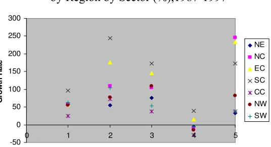
Figure 2. Labor Productivity Growth Rate by Region by Sector (%),1987-1997

-50 0 50 100 150 200 250 300

0 1 2 3 4 5

Industry

Gr

o

w

th

R

a

te

NE

NC

EC

SC

CC

NW

We also should note that the high dispersions of labor productivity levels within

the same sector among regions are likely due to the very different mix of industries below

the sector level used in our analysis, rather than to a strong variety of labor productivity

levels of single products. Given the high level of aggregation in the MRIO tables, we

often had to remind ourselves of this fact, particularly when analyzing results for the

Manufacturing and Service sectors. Both are aggregates of a large number of

heterogeneous industries. Also in the course of the analysis we found ourselves recalling

the sage advice of Dietzenbacher et al. (2000) that sectors with the highest productivity

levels ought not to be automatically interpreted as being the technologically most

advanced. This is because labor productivity levels are also affected by capital-labor

ratios that partly depend upon relative factor prices. Thus, we often found that the

employment share of the sector with the lowest labor productivity level among the five

sectors was greater than the one with highest labor productivity. This implies that labor

productivity can increase with regional specialization, which causes the demand for labor

to decrease.

Table 4 presents summary statistics for the seven regions in China from 1987 to

1997. Central China, Southwest China and Northwest China, which start out with low

initial labor productivity endowments, have relatively low productivity growth during the

ten following years. On the contrary, the other three regions including North China, East

China and South China develop with a surprising speed. The Northeast, as we can

observe from Table 3, maintains a relatively low growth rate throughout the period,

despite a higher initial labor productivity endowment.

From Figure 2 we can see that almost all sectors in every region experienced

positive labor productivity growth rates during the study period. An exception is Trade

and Transportation. Labor productivity for that sector even decreased across five of the

regions. The reason for this may be manifold. First, it can probably be attributed to

inaccuracies in China’s statistical system. Hioki and Okamoto (forthcoming) point out

some problems about China’s statistical information system for transportation industry, in

particular they focus upon the consistency between transportation statistics and other

national economic statistics. Second, the Trade and Transport sector itself in general does

the other four sectors. Also, since data on total hours worked by sector were not available,

the employment data we use represents the total number of workers engaged in the

industry including temporary employees. Thus, the issue could be more fundamental.

That is, it may well be that, as elsewhere in the world, the sector experienced a rapid

increase in its use of part-time and seasonal employees. This would, of course, lead to

some bias in our analysis.

For North China, the Service sector is of vital importance. It experienced an

increase in its labor productivity growth of more than 100% during the period of study,

although several other sectors also have such strong performance. All sectors in East

China performed above average, and the region especially excelled in Services,

Manufacturing, and Construction. South China owes most of its aggregate productivity

increase to Manufacturing, but Construction and Service also contributed. Central China

things appear to be far less sanguine with almost all its sectors lagging behind those in

other regions. The growth in the Northwest can largely be attributed to Construction as its

labor productivity ranks top among all sectors in this region. This can probably be

attributed to the national government’s West Development Strategy. The Southwest

performed best in Manufacturing, and sectors in Northeast did not show much change.

To this point, we attempted to relate a general understanding about temporal and

spatial variations in China’s labor productivity from 1987 to 1997. Both labor

productivity and its growth rate differ across regions and industries. But we have not yet

ascertained what contributed to the total change. The following decomposition analysis is

our attempt to make this determination.

4.2 Decomposition results

The results of the application of decomposition for Equations (1) and (2) are

reported in Table 5 and 6. Table 5 displays the perspective of regions by aggregating

sectors, and Table 6 focuses on sectors by aggregating regions.

Based on the MRIO data, labor productivity in China increased by 90.8 percent

during the 1987-1997 period—an annualized growth rate of 6.7%. The increase was

mainly caused by a decrease in labor used per unit of gross output. It alone accounts for

decompositions). This effect was partly offset by a shrinking of value added’s share of

total inputs—a reduction of about 20 percent.

The decrease of labor input per unit of gross output indicates the adoption of

labor-saving processes, which resulted in the substitution of capital for labor or

reductions in disguised unemployment. Much of the change was undoubtedly induced via

market pressures as China engaged more fully in the world marketplace as suggested by

Tybout (1992) and the many other researchers engaged in work on the exports under a

regime of heterogeneous establishments.

Although not directly detectable from the results in Table 5, we should note that

the length of the work week was substantially reduced in 1994 and again in 1995. Prior to

March 1, 1994, the work week was 48 hours long; on that date it was reduced to 44 hours.

The official work week was reduced by 4 hours more to 40 hours starting on May 1, 1995.

This means that if one is really interested in measures of labor productivity growth and

labor input per unit of gross output that are based on a labor-hour rather than a job basis,

the numbers in Table 5 and Table 6 are clear underestimates. We should note that value

added per unit of gross output was, in many cases, also caused by the same labor-saving

effect as well as being laid open to the ravages of pressures from increasing exposure to

world markets. In particular, the latter undoubtedly induced tax and profit shares in China

to decrease between 1987 and 1997, by about 5 percent.

Changes in input structure (factor 3) and in final demand (factor 5) have a net

positive effect on the growth of labor productivity. While changes in interregional trade

(factor 4) seems to have yielded no contribution to the labor productivity at national level,

change in final demand provided a greater impetus for labor productivity growth than did

change in intermediate input structure—i.e., change in technology and in the mix of

Table 5 Labor Productivity Decomposition Results by Region

Region Total1 Factor 12 Factor 2 Factor 3 Factor 4 Factor 5

NE 1.401 0.739 0.757 0.748 1.853 1.801 1.827 0.969 0.995 0.982 0.989 0.978 0.983 1.008 1.013 1.010 NC 2.162 0.805 0.795 0.800 2.327 2.104 2.213 1.058 1.111 1.084 1.007 1.019 1.013 1.074 1.138 1.106 EC 2.426 0.758 0.771 0.764 2.797 2.351 2.564 1.077 1.165 1.120 0.974 0.970 0.972 1.070 1.164 1.116 SC 2.934 0.792 0.834 0.813 2.877 2.418 2.638 1.100 1.151 1.125 1.031 1.059 1.045 1.141 1.216 1.178 CC 1.484 0.835 0.839 0.837 1.513 1.461 1.487 0.995 1.007 1.001 1.034 1.017 1.025 1.053 1.091 1.072 NW 1.683 0.863 0.863 0.863 1.800 1.761 1.780 0.917 1.008 0.961 0.958 0.962 0.960 1.090 1.100 1.095 SW 1.786 0.836 0.849 0.842 1.790 1.764 1.777 1.113 1.108 1.110 0.962 0.974 0.968 1.092 1.098 1.095 China 1.908 0.79851 0.810 0.804 2.0066 1.812 1.907 1.0504 1.0889 1.069 0.995 0.9989 0.997 1.0912 1.1635 1.127 Note: 1. Ratio of labor productivity in 1997 to that in 1987;

2. First columns of each factor refer to results of Equation (1) and second columns refer to results of Equation (2) and third columns refer to Fisher indexes, which is the geometric average of the first two indexes.

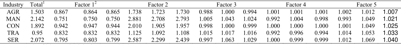
Table 6 Labor Productivity Decomposition Results by Sector

Industry Total1 Factor 12 Factor 2 Factor 3 Factor 4 Factor 5 AGR 1.503 0.867 0.864 0.865 1.738 1.723 1.730 0.988 1.000 0.994 1.001 1.001 1.001 1.002 1.012 1.007 MAN 2.142 0.751 0.750 0.750 2.881 2.708 2.793 1.005 1.043 1.024 0.992 1.004 0.998 0.993 1.049 1.021 CON 1.892 0.942 0.947 0.944 2.010 1.905 1.957 0.998 1.000 0.999 1.000 1.000 1.000 1.001 1.049 1.025 TRA 0.95 0.832 0.832 0.832 1.125 1.092 1.108 1.015 1.017 1.016 0.992 0.996 0.994 1.014 1.053 1.033 SER 2.072 0.795 0.803 0.799 2.587 2.299 2.439 0.997 1.063 1.029 1.000 0.999 0.999 1.012 1.069 1.040 Note: 1. Ratio of labor productivity in 1997 to that in 1987;

The findings summarized for each of the seven regions are quite similar to those

for the China as a whole. Decreased labor input per unit of gross output contributes the

most to labor productivity growth followed by changes in final demand. Input structure

tends to rank third and fourth as a key factor. Reduction in the ratios of value added per

unit of gross output markedly dampened the labor productivity increases.

Our result differ quite a bit from those of Dietzenbacher et al. (2000) in that they

found the effects from both changes in intermediate structure and trade and changes in

final demand to have no perceptible effect on growth of labor productivity for any of the

Euro-6 countries they analyzed. While our findings for change in interregional trade were

similar, those for final demand were not. Indeed, change in final demand nearly

consistently contributed substantially to labor productivity growth in each of the seven

regions and five industries in the MRIO tables we used to analyze China’s economy.

Thus, in our case both the change in final demand and in intermediate input structure

appear to have fostered growth in labor productivity in China from 1987 to 1997. We also

found that value-added’s share of gross output reduced its contribution to labor

productivity growth by about 20 percent for each of China’s regions. Dietzenbacher et al.

(2000) found a less dramatic 10 percent reduction in this factor’s contribution to labor

productivity growth. The difference is undoubtedly due to world’s openness to rapidly

increase trade with China. While the Euro-6 also benefited from a greater openness in

trade during the study period employed by Dietzenbacher et al., those countries already

were among the world leaders in adopting technological innovations and engaged heavily

in international trade prior to the study period. Hence, the economic pressures of freer

trade were not nearly so heavily felt in Europe between 1975 and 1985 as they were in

China between 1987 and 1997.

When we look at the factors by region, it can be inferred that the high labor

productivity growth in North China, East China, and South China derives largely from

large decreases in the use of labor per unit of gross output. In the same three regions plus

the Southwest, changes in intermediate input structure also improved labor productivity

by about 10 percent. Interregional trade had a clear positive effect on North China, South

Northeast, East China, Northwest, and Southwest and—about 2, 3, 4 and 3 percent,

respectively.

We made several cursory investigations as attempts to explain why the

interregional trade effects were positive for some regions while negative for others.

Unfortunately, each approach only supported a subset of the regions. In one approach we

examined each region’s in-and out-flows with imports calculated from perspectives of

both using and producing industries. Analyses of these data revealed that Manufacturing

was by far the dominant trading sector for all regions in both periods. We also compare

the change in labor productivity of in- and outflows (calculated for using industries using

a weighted average) for the sectors by region. We hypothesized that regions’ sectors with

higher labor productivities for their outflows than their inflows should yield positive

effects on labor productivity and, of course, that opposite results should yield negative

productivity effects. It proved to be the case for five of the seven regions: East China and

Central China were anomalies. We also calculate each sector’s outflow share by region

with the hypothesis that interregional trade effects would be positive when the outflow’s

share in high-productivity sectors increases between 1987 and 1997. Again, for all but

East China the hypothesis appeared to ring true. Thus despite a modicum of success our

search for explanations of the results obtained, it is clear that some further research is

required to ascertain more precisely what factors contributed to the interregional trade

effects we obtained.

Factor 5, change in final demand, has a major effect on all the regions but the

Northeast. We found that, from 1987 to 1997, the Northeast’s final demand share in

Trade and Transportation increased from 1.6 percent to 7.4 percent. As we mentioned

above, labor productivity of this sector decreased. Thus, it may be a major reason that the

effect of final demand is less important in Northeast.

From Table 6, observe that labor productivity increased by an astounding 114

percent from 1987 to 1997 in Manufacturing and 107 percent in the Service sector! At the

same time, as stated earlier, productivity in Trade and Transportation declined. Most

sectors in China experienced larger rises in labor productivity and drops in value-added

per unit of gross output from 1987 to 1997 than did their counterparts in the Euro-6

derive mainly from declines in labor input per unit of gross output. Skyrocketing labor

productivity in the Manufacturing and Service sectors are largely caused by this. The

second most important factor across the sectors is the change in value added per unit of

output. Although it is negative and, hence, dampened productivity growth.

As has been the story throughout this paper, the input structure and changes in

final demand had smaller effects compared with the first two factors. Their magnitudes

are, nonetheless, significantly larger than the corresponding factors for the Euro-6

countries during the 1975-1985 period, as estimated by Dietzenbacher et al. (2000). The

effects of these two factors are negligible for Agriculture, but make up about 2.4 percent

and 2.1 percent, respectively, of productivity change for Manufacturing and about 1.6

percent and 3.3 percent, respectively, of productivity change for Transportation and

Trade. Input structure had no apparent effect on the productivity of Construction, which

implies that there was no significant technology change in the China’s Construction

sector during the study period. Changes in the pattern of interregional trade almost had no

effect on the productivity of the sectors; there may be some explanations for this.

Construction and Service sectors do not generally produce a traded good or service.

Dietzenbacher et al. (2000) also give some reasons for this in their paper. Compared to

other sectors, change in final demand for the Service sector contributed most to overall

sectoral productivity growth, and at 2.9 percent change in its input structure also yielded

relatively large effects compared to other sectors.

Comparing Table 5 to Table 6, we can make further inferences. The first two

factors tend to yield the largest effects, while effects from the last three factors tend to be

smaller. The lack of effect from changes in input structure is readily explained by the

generally slow pace of technology change within a ten-year timeframe. Work by Carter

(1970) and others have long suggested that ten years is insufficiently long to change

average industry structure even in innovative industries. That the factors have more effect

upon regions than upon sectors implies that different intrasectoral structures exist across

the regions and, thus, that subsector mix issues generate some substantial share of the

regional disparity in labor productivity.

Along the way we have compared our results for China with those by

comparison and enlightens us about the relative magnitude of labor productivity growth

as well as provides some background for identifying further causes of interregional

disparities in productivity growth. In summary we have found that all factors tended to

provide impetus for labor productivity growth in China between 1987 and 1997 than they

did in Euro-6 countries from 1975 to 1985. This finding was most poignant for input

structure, interregional trade, and final demand changes. These key differences could

have more to do with the way the tables were built rather than from the economic

changes that the two global regions were undergoing during the respective study periods.

Dietzenbacher et al. (2000) note that the input-output tables they used were constructed

using exchange rates among the countries rather than purchasing power parity (PPP)

conversions. Since our analysis focuses on regions of a single country, PPP versus

exchange-rate conversion is a non-issue. For similar reasons, transaction costs of trade

among regions of a single country are naturally smaller than they are for trade among

different countries. That is, the flow of commodities and services should be relatively

frictionless for China, which is not the case for the Euro-6. Thus, China’s economic

reformation, which started in 1978, had better ability to induce sweeping technology

change during the second decade following that reform that did the formation of the

European Union. Most studies of technology change have been undertaken in relatively

stable economies or in economies in decades when trade and information exchange were

slower on the uptake.

5. CONCLUSIONS

Few papers have studied the factors contributing to changes in labor productivity

with multiregional input-output tables. This is particularly the case for China. In this

paper we use two multiregional input-output tables and disaggregated employment data

to examine change in labor productivity growth for seven regions and five sectors of the

Chinese economy between 1987 and 1997. We decompose the potential causes of change

in labor productivity into five partial effects. We find that the increase of labor

productivity for regions and sectors in China mainly comes from the decreasing labor

input per unit of gross output and from changes in value added’s share of gross output.

Aggregate production mix, interregional trade, and final demand also have important but

We found that the factor effects were larger by region than by industry. This

suggests that regions’ subsector industry mixes also play a role in causing interregional

disparities in GDP production. The paper also shows that all the factors displayed larger

effects in China from 1987 to 1997 then did Euro-6 countries from 1975 to 1985.

Like other decomposition methods, this approach deals only with proximate

causality, and thus we give our understanding based on the knowledge of institutions,

history, policy, and so on. Due to relatively poor economic statistical reporting, especially

for the early years, we can only present a rather aggregate decomposition of China’s

labor productivity among regions and sectors. Accordingly, some in-depth and

more-detailed insight may not be detected. Nonetheless, our analysis presents a fresh

perspective on an issue of national and possibly even international interest. We therefore

hope our work induces others to make further investigations into China’s interregional

References

Albert Keidel, 2007. “China’s Economic Fluctuations and their Implications for the Rural Economy,” available at

http://www.carnegieendowment.org/files/keidel_report_final.pdf

Meng, Bo and Chao Qu, 2007. “Application of the Input-Output Decomposition Technique to China’s Regional Economies,” IDE Discussion Papers, No.102, available at

http://ir.ide.go.jp/dspace/bitstream/2344/552/1/ARRIDE_Discussion_No.102_me ng.pdf

Carter, Anne. 1970. Structural Change in the American Economy. Cambridge, Massachusetts: Harvard University Press.

Cai F., Wang D. and Du Y., 2002. “Regional Disparity and Economic Growth in China The Impact of Labor Market Distortions,” China Economic Review, 13: 197–212.

China’s State information Center .Multi-regional Input-output Table for China, Social Science Academic Press (China) 2005.

Démurger, Sylvie. 2001. “Infrastructure Development and Economic Growth: an Explanation for Regional Disparities in China?” Journal of Comparative Economics, 29: 95-117.

Démurger, Sylvie, Jeffrey D. Sachs, Wing T. Woo, Shuming Bao, Gene Chang and Andrew Mellinger. 2002. “Geography, Economic Policy and Regional Development in China,” 2002. NBER Working Paper, No. 8897.

Demurger, Sylvie, Jeffrey D. Sachs, Wing T. Woo, Shuming Bao and Gene Chang. 2002. “The Relative Contributions of Location and Preferential Policies in China’s Regional Development: Being in the Right Place and Having the Right Incentives,” China Economic Review, 13, 444-465.

Dietzenbacher, Erik, Alex R. Hoen, and Bart Los. 2000. “Labor Productivity in Western Europe 1975-1985: An Intercountry, Interindustry Analysis,” Journal of Regional Science, 40 (3): 425-452.

Dietzenbacher, Erik and Alex R. Hoen. 1998. “Deflation of Input-output Tables from the User’s Point of View: A Heuristic Approach,” Review of Income and Wealth, 44(1): 111-122.

Hioki, Shiro and Nobuhiro Okamoto. forthcoming."How Have China's Intra- and Inter-regional Input-Output Linkages Changed during the Economic Reform," Chapter 6. in Nazrul Islam ed. Resurgent China: Issues for the Future. London: Palgrave MacMillan.

Ichimura, Shinichi and Hui-Jioing Wang. 2003. Interregional Input-Output Analysis of the Chinese Economy. Singapore: World Scientific Publishing Co. Inc.

Li Huaqun and Haynes Kingslay E., “Industrial Structure and Regional Disparity in China: Beyond the Kuznets Transition.” 47th Southern Regional Science Association Annual Meeting in Washington DC

Lin, Justin Yifu and Peilin Liu, 2005. “Development Strategies and Regional Income Disparities in China,” China Center for Economic Research Working Paper No. 2005005, Beijing University.

Liu, Tung and Kui-Wai Li, 2006. “Disparity in Factor Contributions between Coastal and Inner Provinces in Post-reform China,” China Economic Review, 17: 449-470.

National Bureau of Statistics of China (1988-1998), China Statistical Yearbook, Beijing. China Statistics Press.

National Bureau of Statistics of China (1988-1990), China Industry Economy Statistical Yearbook, Beijing. China Statistics Press.

National Bureau of Statistics of China, China Urban Life and Price Yearbook 2006, Beijing. China Statistics Press.

National Bureau of Statistics of China, 1949~2004 China Statistical Data Compilation, 2005, Beijing. China Statistics Press.

Shang Jin, Wei and Yi Wu , 2001. “Globalization and Inequality: Evidence from within China,” NBER Working Paper 8611

Sun, Haishun and Ashok Parikh. 2001. “Exports, Inward Foreign Direct Investment (FDI) and Regional Economic Growth in China,” Regional Studies 35 (3): 187-196. Tybout, James, R. 1992. “Linking Trade and Productivity: New Research Directions,” World Bank Economic Review, 6, 189-211.

Wei, Yehua Dennis. 2000, “Investment and Regional Development in Post-Mao China,” Geojournal, 51(3): 169-179.

APPENDIX

Table of price index

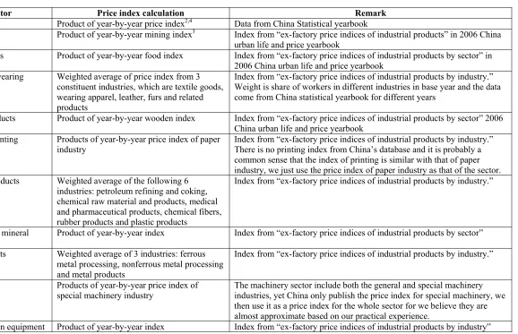
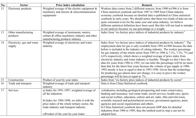
No. Sector Price index calculation Remark

1 Agriculture Product of year-by-year price index2,4 Data from China Statistical yearbook

2 Mining Product of year-by-year mining index3 Index from “ex-factory price indices of industrial products” in 2006 China urban life and price yearbook

3 Food products Product of year-by-year food index Index from “ex-factory price indices of industrial products by sector” in 2006 China urban life and price yearbook

4 Textile and wearing apparel

Weighted average of price index from 3 constituent industries, which are textile goods, wearing apparel, leather, furs and related products

Index from “ex-factory price indices of industrial products by industry.” Weight is share of workers in different industries in base year and the data come from China statistical yearbook for different years

5 Wooden products Product of year-by-year wooden index Index from “ex-factory price indices of industrial products by sector” 2006 China urban life and price yearbook

6 Paper and printing Products of year-by-year price index of paper industry

Index from “ex-factory price indices of industrial products by industry.” There is no printing index from China’s database and it is probably a common sense that the index of printing is similar with that of paper industry, we just use the price index of paper industry as that of the sector. 7 Chemical products Weighted average of the following 6

industries: petroleum refining and coking, chemical raw material and products, medical and pharmaceutical products, chemical fibers, rubber products and plastic products

Index from “ex-factory price indices of industrial products by industry.”

8 Non-metallic mineral products

Product of year-by-year index Index from “ex-factory price indices of industrial products by sector”

9 Metal products Weighted average of 3 industries: ferrous metal processing, nonferrous metal processing and metal products

Index from “ex-factory price indices of industrial products by industry.”

10 Machinery Products of year-by-year price index of special machinery industry

The machinery sector include both the general and special machinery industries, yet China only publish the price index for special machinery, we then use it as a price index for the whole sector for we believe they are almost approximate based on our practical experience.

Table of Price index (Cont)

No. Sector Price index calculation Remark

12 Electronic products Weighted average of the electric equipment & machinery and electric & telecommunication equipments

Workers data comes from 2 different sources; from 1990 to1996 it is from China statistical yearbook and from 1987 to 1989 from China industry economy yearbook because no detailed data is published in China statistical yearbook in early years. We should notice that these two kinds of data are not quite consistent even for the same year and same industry, we believe

different statistical definition have been used. But this will not lead to mistake in our analysis because we use percentage as a weight.

13 Other manufacturing products

Weighted average of instrument, meters, culture & office machinery industry and other manufacturing products industry

Index from “ex-factory price indices of industrial products by industry”

14 Electricity, gas and water supply

Weighted average of electricity and water industry

Index from “ex-factory price indices of industrial products by industry”. The employment data for gas is only available from 1993 to1996 because the data before is included in the industry of coking industry. The worker percentage for gas industry of the whole sector from 1993 to 1996 is 7.2%, 7.3%, 7% and 6.6% respectively, which shows a weighted average of price index from electricity industry and water industry is feasible. Though we don’t have the data for years from 1986 to 1992, we can infer the percentage will be no more than that for the latest four years because the volume of gas supply in 1986-1992 mostly is less or equal to that in 1993-1996. Given that the technology for producing gas almost does not change, it is easy to prove the worker percentage will be less or equal to 7%.

15 Construction Product of year-by-year index Index from “ex-factory price indices of industrial products by sector” 16 Trade and transport Weighted average of trade and transport

industry

Data is from China Statistical yearbook.

17 Services a) Index for 1991-1997, weighted average of all the industries

b) Index for 1988-1990, we infer it with the price index of the whole tertiary sector, the trade industry and transport industry

c)Product of the year-by-year index

a)Industries including geological prospecting and water conservancy, banking and insurance, real estate trade, social services, health care, sports and social welfare, education, culture and art, radio, film and television, scientific research and polytechnical services, government agencies, party agencies and social organizations and others.

The data we used to calculate the price index come from the China Statistical

Yearbook, the China Urban Life and Price Yearbook, and the China Industry Economy

Yearbook. We were unable to find a proper price index for agriculture and tertiary

industries (both for the aggregate Service sector and its finer component industries) in the

China Urban Life and Price Yearbook or other data bases for China. Nonetheless, we

needed to calculate them using existing data. Thus we created an implicit GDP price

deflator using data in the China Statistical Yearbook. We calculated it by taking the ratio

of nominal GDP to real GDP for both 1987 and 1997, and dividing the 1997 result by the

1987 value.

For industries of the Manufacturing sector in the 1997 MRIO table, we selected the

most appropriate price index from factory price indices of industrial products”,

“ex-factory price indices of industrial products by sector” or “ex-“ex-factory price indices of

industrial products by industry” in the China Urban Life and Price Yearbook. (For the

“ex-factory price indices of industrial products by sector,” see the definition of the

industry in the appendix to the 1988 China Industry Economy Yearbook.) Naturally, if an

index was perfectly consistent with an industry in the 1997 MRIO table, we used it

directly: Otherwise, we generated a price index based on weighting of several finer

industries’ indices. As weights we used GDP share for agriculture and tertiary industries.

Due the greater detail in the manufacturing industries and the lack of equivalently

detailed GDP data, we used worker shares. We used base-year shares as weights.

Industrial reporting in China changed during the ten years that we study. For

example, the foraging industry was a distinct industry before 1993: It was merged

subsequently into the food-processing industry. Similarly, the coke-making industry was

a distinct industry before 1990 and was subsequently merged into the petroleum-refining

and coke-making industry. The industrial arts industry was included within the “other

manufacturing” industry prior to 1990 and was reported separately afterward. All of these

anomalies were accounted for inasmuch as data permitted.

In several cases, we were forced to use a combination of data on manufacturing

workers for both 1987 and 1988 from the China Statistical Yearbook as weights. We note

establishments that were collectively owned. In 1988 about 98.8% of all Chinese

manufacturing workers were employed by such organizations. Similarly, the 1988 China

Statistical Yearbook reports workers counts by industry only for establishments

collectively owned above the county level. In 1987 these organizations comprised more

than 88.4% of all Chinese manufacturing workers. Despite this, our use of shares as

weights should minimize any inherent bias, except in those industries especially sensitive