Trading volume and the number of trades:a comparative study using high frequency data

Lancaster University Management School

Working Paper

2007/014

Trading volume and the number of trades:

A comparative study using high frequency data

Marwan Izzeldin

The Department of Economics Lancaster University Management School

Lancaster LA1 4YX UK

© Marwan Izzeldin

All rights reserved. Short sections of text, not to exceed two paragraphs, may be quoted without explicit permission,

provided that full acknowledgement is given.

The LUMS Working Papers series can be accessed at http://www.lums.lancs.ac.uk/publications/

Trading Volume and the Number of Trades:

A Comparative Study Using High Frequency Data

Marwan Izzeldin

Department of Economics, Lancaster University, Lancaster LA1 4YX, UK. ([email protected])

March 2007

Abstract

Trading volume and the number of trades are both used as proxies for market activity, with disagreement as to which is the better proxy for market activity. This paper investigates this issue using high frequency data for Cisco and Intel in 1997. A number of econometric methods are used, including GARCH augmented with lagged trading volume and number of trades, tests based on moment restrictions, regression analysis of volatility on volume and trades, normality of returns when standardized by volume and number of trades, and Correlation analysis using volatility generated from GARCH and realized volatility. Our results show that the number of trades is the better proxy for market activity.

Keywords: Trading volume; number of trades; realized volatility, GARCH

I. Introduction

The volatility-volume relation is central to many models in finance and economics. Since the early 1970s, the relation between trading volume and stock prices volatility has been widely investigated in an impressive body of empirical and theoretical literature. The first treatment of the relation goes back to Osborne (1959) in his attempt to model the stock price change as a diffusion process with volatility related to the number of transactions. This was followed by the work of Ying (1966) and Crouch (1970), who find a statistically significance positive correlation between absolute returns and daily volumes for both market indices and individual stocks. Clark (1973) finds a positive relation between squared returns and aggregated volume using daily data from the cotton futures market. Westerfield (1977) finds a similar relation in a sample of returns and volumes for a number of common stocks, as do Tauchen and Pitts (1983) using daily data from the Treasury Bill futures market. Epps and Epps (1976) find a positive relation between the sample variances of returns at given volume levels using transactions from 20 stocks. Harris (1986, 1987) finds a positive correlation between volume and the square of the price change using daily data. Moreover Karpoff (1987, 1988), Lamaourex and Lastrapes (1990, 1994), Liesenfeld (1998, 2001), Richardson and Smith (1994) and Tauchen and Pitts (1983) have all emphasized the role of volume as an activity variable.

unforeseen information flow process. The MDH also tells us that volume is the best proxy for market activity; hence we expect the correlation between volume and any volatility proxy to be an increasing function of the accuracy of the volatility measure in use. However, this is not the case with the data we use here where the number of trades is found to show higher correlation with realized volatility than volume, which in turn suggests a volatility-number of trades relation as opposed to the volatility-volume relation implied by the MDH.

The support for the number of trades that we find in this paper is in line with a growing literature which tends to emphasize the role of the number of trades over volume. For example, March and Rock (1986) finds that the net number of trades has similar explanatory power as net volume. Jones et al.(1994) argue that trading volume has no informational content beyond that contained in the number of trades. As a result they suggest the use of the number of trades as a substitute for volume. More recent evidence can be found in the work of Easley and O'Hara (1992), Easley et al. (1997), Hasbrouk (1999).and Ané and Geman (2000).

out in Harris (1986) and Ané and Geman (2000). Moreover we consider correlation analysis by which we look at the correlation between volume, the number of trades and volatility generated from a variety of commonly used GARCH models - exponential GARCH, threshold GARCH, GARCH in-the-mean, fractional GARCH, fractional EGARCH, two components GARCH - and realized volatility.

The outline of this paper is as follows. In Section II, we discuss the data and the econometric procedures to be used. In section III, we discuss our findings. We present our conclusions in section IV.

II. Data and Methodology

We use the Cisco and Intel high frequency data for 1997 as used in Ané and Geman (2000). We did not have access to Reuters - the source used by Ané and Geman (2000), so we use data from the Wharton Research Data Services

website. We calculate the intra day (9.30 am to 4 pm) returns ( ), volume ( )

and the number of trades ( ) at the 10, 30 and 60 minute and daily time

intervals.

t

r v_t

t

n

We consider a number of econometric procedures / methods as previously used to investigate the volatility-volume and volatility-number of trades relationships. These methods are described below.

Andersen (1996), and Liesenfeld (1998, 2001).and is based on testing the moment restrictions implied by the MDH model using the Generalized Method of Moments (GMM) J- test of overidentifying restrictions.

The MDH assumes that, conditional on the information flow , returns

and the observed "market activity" (volume, log volume, the number of trades

etc.) are independently and normally distributed as:

t

i r_t

t a (1) 2 2 0 | , 0 t t t t

r t r t t

t

t a t a t

i i

r

i N

a i i

µ σ µ σ ⎛⎛ ⎞ ⎛ ⎞⎞ ⎛ ⎞ _⎜ ∼ ⎜ ⎟ ⎜ ⎜ ⎟ _{⎜⎜ ⎟ ⎜} ⎝ ⎠ _{⎝⎝ ⎠ ⎝ ⎠}⎟⎟⎟_⎠⎟, 3 3 i i m m 3 i 3 r 3 a 2

The model implies a set of moment restrictions that can be imposed on the data and evaluated using the GMM J-test of over-identifying restrictions. We consider the moment restrictions set out in equation 4 of Richardson and Smith (1994, p. 106) which can be written as follows:

(2)

2

2

1 1

2 2

2 1 2

2 3

3 2

1 1

2 2

2 1 2

2 3

3 2

11 2

2 2

12 2 3

2 2

21 2 3

3

3 r i

r

r i i r r r i

r r r a i

a

a i i a a r i

a a a ra i

r a

ra i i a r a r ar i i

r a r a

m m

m m m

m m m

m m

m m m

m m m

m m

m m

m m

µ

σ µ

µ σ µ

µ

σ µ

µ σ µ

µ µ

σ µ σ µ

σ µ σ µ

= = + = + = = + = + = = + = +

where, denote the first three (central) moments of information,

denote the first three unconditional (central) moments of returns,

denote the first three unconditional (central) moments of activity and

denote the co-variances between and . 1,..., i m m 1,..., r m m 1,..., a m m 2 11, 12 , 21

ra ra ar

Murphy and Izzeldin (2007) point out, the parameters µ_rand σ_r2are only

identified up to scale since is not observed. Suppose is replaced by with

so that become t

i i_t κi_t

0

κ > m₁i,...,m₃i κm₁i,...,κm₃iin the moment conditions. Then

/ r

µ κ and σ κ_r2/ satisfy the new moment conditions. Thus µ σ_r, _r2 and cannot

be identified separately. To overcome this problem, we normalize the mean of

unobserved information flow process to one. Following normalization, the

remaining system consists of nine moment conditions and six parameters to be

estimated ( ). This leaves three over-identifying restrictions

which are evaluated using the J-test of over-identifying restrictions. For example, if J > 7.815, then we can reject the moment restrictions at the 5 % level. The activity variable whose moment restrictions best fit the data, can be taken as a good proxy of market activity. In other words, we seek to establish whether a volatility-volume relation or a volatility-number of trades is appropriate for the volatility-activity relation implied by the MDH.

1

i

m

1

i

m

2 2 2 , , , , i, r a r a m m

µ µ σ σ ₃i

We consider the basic GARCH model outlined in Lamaourex and Lastrapes (1990), but with the mean equation given by

t

r = +c σ_tu_t (3)

and the three variance equations as shown below

2 2

0 1 1 2

t rt

2 1

t

σ =α α+ ₋ +α σ ₋ (4a)

2 2 2

0 1 1 2 1 3

t rt t

σ =α α+ − +α σ− +α vt−1

1

t

n

(4b)

2 2 2

0 1 1 2 1 4

t rt t

σ =α α+ ₋ +α σ ₋ +α ₋ (4c)

We then select the model which best fits the data using the Akaike information criterion (AIC), the significance of the coefficients on v_t−1 and n_t−1,

and the level of persistence given by the sum α α₁+ ₂.

The third method involves comparing the performance of volume and the number of trades in explaining volatility changes. We consider the regressions outlined in Jones et al. (1994) and Ané and Geman (2000) which are as follows:

12

1

ˆ_{t t j t j}

j

s a β v ρ s₋ e

= t

= + ∆ +

∑

12

1

ˆ_{t t j t j}

j

s b γ n ρ s₋ u

=

t

= + ∆ +

∑

12

1

ˆ_{t t t j t j}

j

s c β v γ n ρ s_{− t}

=

η

= + ∆ + ∆ +

∑

where a, b and c are constants, ∆v_t and ∆n_t are the first differences of volume

To generate , we run a regression of the return over 12 lagged returns as

shown in equation 6 below: ˆ_t

s rt

12 1

t j j t

r = +α

∑

We then define sˆ_t

ˆ

2 ˆ

t t

s = π ε (7)

The standardization

2

π

follows from an elementary result on the Gaussian

distribution which asserts that if 2

(0, )

X ∼N σ , then E X

( )

In the fourth method we test one of the assumptions under the MDH which asserts that returns standardized by a good proxy for activity is normally distributed. Clark (1973) shows that returns subordinated/standardized using volume is normally distributed. Ané and Geman (2000) claims that returns standardized by the number of trades are normal. In our exercise we consider returns standardized by volume and returns standardized by the number of trades. The best activity proxy is the one which achieves a higher level of normality for the standardized returns.

Finally, we look at the correlation of volume and trades with volatility

generated from GARCH

(

)

(

)

GARCH

(

)

(

)

fractional exponential GARCH

(

)

(

)

(

)

Bollerslev et al. (1994), Engle (2001) and Glosten (1993). We also consider the correlation between volume, trades and realized volatility. Realized volatility is defined as the sum of the intra-day squared returns which, in the absence of micro-structure effects, provides an unbiased and accurate measure of volatility. See, Andersen. et al. (2001) and Barndorff-Nielsen and Shephard (2001) for example. The realized volatility in our case is constructed by summing 5 minute intra-day squared returns to the daily interval.

III. Results

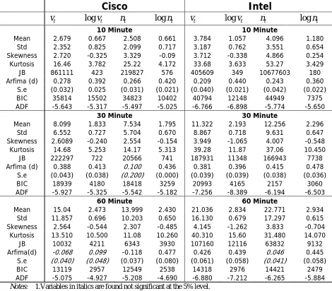
[ Table 1 around here]

Table 1 reports some statistical properties for Cisco and Intel volumes, log volumes, trades and the number of trades. We scale volume by 1/100000 and the number of trades by 1/100 to make the results comparable. The higher mean

and standard deviation of and for Intel over Cisco, indicate more activity

for Intel. Log and log are more normal relative to and as shown by

the Jarque-Bera test statistic. The table also shows the results for the Autoregressive fractionally integrated moving average, Arfima (p, d, q) model

applied to , and . The fractional differencing parameter “d”

shows higher values for l . High persistence is a stylized fact of a good

volatility model. Hence it follows that a good activity proxy that is highly correlated with volatility should also possess high persistence. Since the number of trades is more persistent than volume indicates that the number of trades has more in common with volatility than volume. The results for and should

t

v nt

t

v n_t v_t n_t

, log , t t

v v n_t logn_t

ogn_t

t

not be taken as definitive? Since the custom is to apply the Arfima for the log series and not the level series.

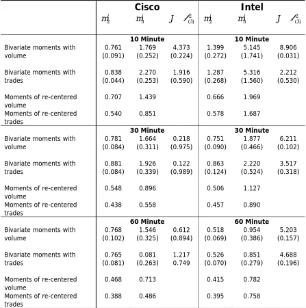
[ Table 2 around here]

Table 2 reports the estimated second and third moments of the

information flow for Cisco and Intel along with the χ₍₃₎2 statistic of the J-test of

over-identifying restrictions. For all the time intervals considered the bivariate moments with trades achieves a lower value for the J-test than that with volume except for the Cisco (60 minute) case, where the results show more support for volume. These results support the MDH model with both trading volume and the number of trades acting as mixing variables, but with greater emphasis on the role of the number of trades.

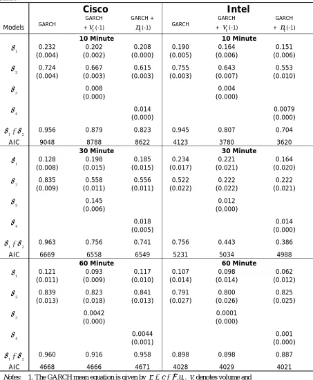
[ Table 3 around here]

Table 3 reports the results of basic and augmented GARCH models, with lagged volume and number of trades. For all cases, GARCH augmented with lagged number of trades shows has lower AIC and lower persistence as given

byα α₁+ ₂ . These results show that the number of trades enhances the fit of the

GARCH model in a similar or better fashion to volume.

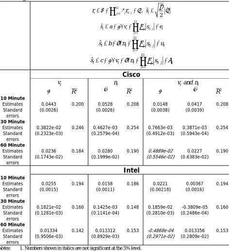
Table 4 reports the results of regression equations (5a, 5b and 5c) as outlined in section II. These provide a method by which to compare the performance of volume and the number of trades in explaining volatility changes. Our results show mixed support for volume and the number of trades. For

example, in the Cisco case, the number of trades shows a higher R2relative to volume at all the time intervals considered. At the 60 minute time interval the combined presence of volume and the number of trades renders volume insignificant. Moreover, regressions 5b and 5c are not statistically different from each other. This shows that the number of trades has more explanatory power than volume. Volume contains no extra information to that provided by the

number of trades. For Intel, volume shows a higher R2 than the number of trades

except for the 60 minute time interval, where R2is higher for the number of trades. Moreover, and similar to the Cisco 60 minute case, the presence of the number of trades and volume renders the coefficient of volume insignificant.

If the Cisco results are taken to be more binding (since they tell the same story across all time intervals) we can conclude that the number of trades is more correlated with the Schwert (1990) volatility measure than is volume. Support for the number of trades is consistent with Jones et al. (1994) and Ané and Geman (2000) both of whom obtain (from a similar framework) results favoring the number of trades.

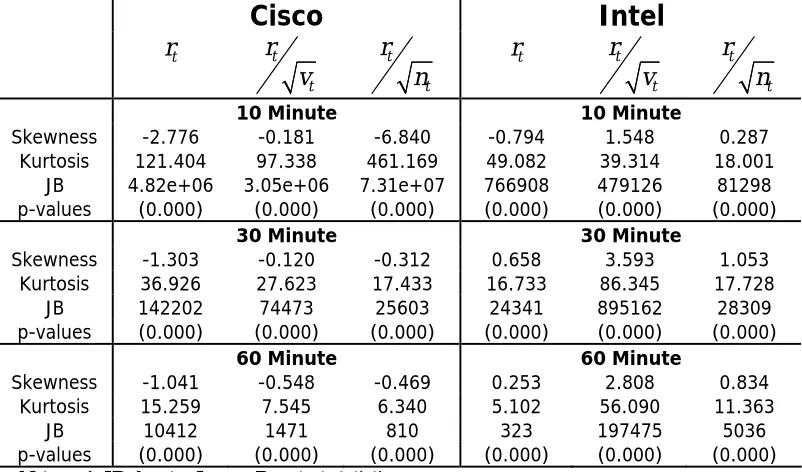
Table 5 reports the results for testing the normality of returns standardized by volume or the number of trades, both rescaled to have a mean of unity. Results obtained show returns standardized by the number of trades are more normal than those standardized using volume, as shown by the Jarque-Bera test statistic. The implication is that the numbers of trades possess more filtration power than volume and hence are able to remove some of the factors causing return non-normality. To the best of our knowledge, no study has managed to recover full returns normality using the number of trades or volume as standardizing variables.

[ Table 6 around here]

Table 6 reports the correlation between the GARCH models, volume and the number of trades at the 60 minute time interval. We consider level correlations and log-correlations. For Cisco, level correlation shows that the number of trades is more closely correlated with GARCH models volatility than is volume. On the contrary, the log-correlation results show that volume is more correlated with these models. In the Intel case, results are mixed. At the level correlation most GARCH models show a higher correlation with the number of

trades than with volume, with the exception ofσ_fegarch. Using log correlation,

garch

σ , σ_tgarch, and σ_pgarch shows a higher correlation with the number of trades

than with volume, whereas σegarch, σfgarch, σfegarch, σ2garch are more correlated

[ Table 7 around here]

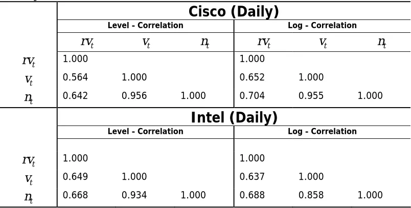
Table 7 shows the correlation between realized volatility, volume and the number of trades. Our results show that realized volatility is more correlated with the number of trades than with volume. In contrast with the correlation for GARCH models, this result holds for both level and log-correlation. Given that realized volatility is considered more accurate than GARCH generated volatility, the results in table 7 have greater credibility: the number of trades is a better proxy for market activity than volume.

IV. Conclusion

A number of econometric methods including GARCH augmented with lagged volume or number of trades, Tests based on moment restrictions and Correlation analysis using volatility generated from GARCH and realized volatility are considered to decide which is the more appropriate measure of market activity: (i) volume or (ii) the number of trades.

Acknowledgments

I wish to thank David Peel, Anthony Murphy, Ivan Paya, Kwok Tong Soo and Gerry Steele for their helpful comments. Any errors are the author’s responsibility.

References

Andersen, T . G. (1996) Return volatility and trading volume: An information flow

Interpretation of stochastic volatility, The Journal of Finance,51 (1), 169-204. Andersen T. G., T. Bollerslev, F. X. Diebold & H. Ebens (2001) The distribution of

realised stock return volatility, Journal of Financial Economics,61, 43-76.

Ané, T. & H. Geman (2000) Order flow, transaction clock, and normality of asset

returns, The Journal of Finance, 55(5), 2259-2284.

Barndorff-Nielsen, O. E. & N. Shephard (2002) Econometric analysis of realized volatility and its use in estimating volatility models, Journal of the Royal

Statistical Society Series B 64, 253 - 280.

Bollerslev, T., Chu R.Y. & K. F. Kroner (1994) ARCH modeling in finance: A selective review of the theory and empirical evidence, Journal of Econometrics 52, 5-59.

Clark, P. K. (1973) A subordinated stochastic process model with finite variance for speculative prices, Econometrica, 41(1), 135-155.

Crouch, R. L. (1970) A nonlinear test of the random-walk hypothesis, American Economic Review,60, 199-202.

Easley, D. & M. O.Hara (1992) Time and the process of security price adjustment, The Journal of Finance,47 (2), 577-605.

Easley, D., N. Kiefer & M. O.Hara (1997) One day in the life of a very common stock, Review of Financial Studies,10, 805- 835.

Engle, R. F (2001) GARCH 101: The use of ARCH/GARCH models in applied economics, Journal of Economic Perspectives,15, 157 - 168.

Epps, W. & M. Epps (1976) The stochastic dependence of security price changes and transaction volumes: implications for the mixture of distribution hypothesis,

Econometrica, 44 (2), 305-321.

Glosten, L. R., R. Jagannathan & D. E. Runkle (1993) On the relation between the expected value and the volatility of the nominal excess returns on stocks.,

Journalof Finance, 48 (5), 1779-1801.

Harris, L. (1986) Cross-security tests of the mixture of distributions hypothesis,

Journal of Financial and Quantitative Analysis,21, 39-46.

Harris, L. (1987) Transaction data of the mixture of distributions hypothesis,

Journal of Financial and Quantative Analysis. 22(2), 127-141.

Hasbrouk, J.(1999) Trading fast and slow: Security market events in real time, Working Paper, New York Stock Exchange.

Jones, M., G. Kaul & M. Lipson (1994) Transactions, volume and volatility,

Review of Financial Studies, 7(4), 631-651.

Karpoff, J. M. (1987) The relation between price changes and trading volume: A survey, Journal of Financial and Quantative Analysis, 22(1), 109-126.

Karpoff, J. M. (1988), .Costly short sales and the correlation of returns with volume, Journal of Financial Research, 11, 173-188.

Lamaourex, C. G. & D. Lastrapes (1990) Heteroskedasticity in stock return data: Volume versus GARCH effects, Journal of Finance, 45, 221-229.

Lamaourex, C. G. & D. Lastrapes (1994) Endogenous trading volume and momentum in stock-return volatility, Journal of Business and Economic Statistics,12, 253-260.

Liesenfeld, R. (1998) Dynamic bivariate mixture models: Modeling the behavior of prices and trading volume, Journal of Business and Economic Statistics, 16, 101-109.

Liesenfeld, R. (2001) A generalized bivariate mixture model for stock price volatility and trading volume, Journal of Econometrics,104, 141-178.

Marsh, T. A. & K. Rock (1986) The transactions process and rational stock prize dynamics, working paper, University of California at Berkeley.

Murphy, A. & M. Izzeldin (2007) Recovering the moments of information flow and the normality of asset Returns, forthcoming, Finance Letters .

Osborne, M. F. M. (1959) Brownian motion in the stock market, Operations Research,7, 145-173.

Tauchen, G. & M. Pitts (1983) The price variability-volume relationship on speculative markets, Econometrica, 51, 485-505.

Westerfield, R. (1977) The distribution of common stock price changes, Journal of Quantative Analysis, 12(5), 743-765.

Table 1. Statistical properties of volume and the number of trades

Cisco Intel

t

v logv_t n_t logn_t v_t logv_t n_t logn_t

10 Minute 10 Minute

Mean 2.679 0.667 2.508 0.661 3.784 1.057 4.096 1.180

Std 2.352 0.825 2.099 0.717 3.187 0.762 3.551 0.654

Skewness 2.720 -0.325 3.329 -0.09 3.712 -0.338 4.866 0.254 Kurtosis 16.46 3.782 25.22 4.172 33.68 3.633 53.27 3.429 JB 861111 423 219827 576 405609 349 10677603 180

Arfima (d) 0.278 0.392 0.266 0.420 0.209 0.440 0.243 0.360

S.e (0.032) 0.025 (0.031) (0.021) (0.040) (0.021) (0.042) (0.022)

BIC 35814 15502 34823 10402 40794 12148 44949 7375

ADF -5.643 -5.317 -5.497 -5.025 -6.766 -6.898 -5.774 -5.650

30 Minute 30 Minute

Mean 8.099 1.833 7.534 1.795 11.322 2.193 12.256 2.296

Std 6.552 0.727 5.704 0.670 8.867 0.718 9.631 0.647

Skewness 2.6089 -0.240 2.554 -0.154 3.949 -1.065 4.007 -0.548 Kurtosis 14.68 5.253 14.17 5.313 39.28 11.87 37.06 10.450

JB 222297 722 20566 741 187931 11348 166943 7738

Arfima (d) 0.388 0.413 0.100 0.436 0.381 0.396 0.415 0.478

S.e (0.043) (0.038) (0.200) (0.000) (0.039) (0.039) (0.038) (0.036) BIC 18939 4180 18418 3259 20993 4165 2157 3060

ADF -5.927 -5.325 -5.542 -5.182 -7.256 -8.389 -6.194 -6.503

60 Minute 60 Minute

Mean 15.04 2.473 13.999 2.430 21.036 2.834 22.771 2.934

Std 11.857 0.696 10.203 0.650 16.130 0.679 17.297 0.615

Skewness 2.564 -0.544 2.307 -0.485 4.145 -1.262 3.833 -0.704 Kurtosis 13.510 10.500 11.08 10.260 40.310 15.60 31.480 14.070

JB 10032 4211 6343 3930 107160 12116 63832 9132

Arfima(d) -0.068 0.099 -0.118 0.477 0.426 0.439 0.046 0.445

S.e (0.040) (0.048) (0.037) (0.080) (0.061) (0.058) (0.041) (0.058) BIC 13119 2957 12549 2538 14318 2976 14421 2479

ADF -5.075 -4.927 -5.208 -4.690 -6.880 -7.212 -6.265 -5.884

Notes: 1.Variables in italics are found not significant at the 5% level.

2. v_t denotes volume, denotes the number of trades., Std denotes standard deviation.,. JB denotes Jarque-Bera test statistic,. BIC denotes Bayesian information criterion, S.e denotes standard error.

t

n

3. Arfima (Autoregressive Fractionally Integrated Moving Average) and d is the fractional differencing parameter.

4. ADF denotes Augmented Dickey Fuller Test. The 5% and 1% critical values are -2.862 and -3.433.

Table 2. Estimated moments of information and J-test of over identifying restrictions

Cisco Intel

2

i

m m₃i J ∼χ₍₃₎2 mi₂ m₃i J ∼χ₍₃₎2

10 Minute 10 Minute

0.761 1.769 4.373 1.399 5.145 8.906 Bivariate moments with

volume (0.091) (0.252) (0.224) (0.272) (1.741) (0.031)

0.838 2.270 1.916 1.287 5.316 2.212 Bivariate moments with

trades (0.044) (0.253) (0.590) (0.268) (1.560) (0.530)

Moments of re-centered

volume 0.707 1.439 0.666 1.969

Moments of re-centered

trades 0.540 0.851 0.578 1.687

30 Minute 30 Minute

0.781 1.664 0.218 0.751 1.877 6.211 Bivariate moments with

volume (0.084) (0.311) (0.975) (0.090) (0.466) (0.102)

0.881 1.926 0.122 0.863 2.220 3.517 Bivariate moments with

trades (0.084) (0.339) (0.989) (0.124) (0.524) (0.318)

Moments of re-centered

volume 0.548 0.896 0.506 1.127

Moments of re-centered

trades 0.438 0.558 0.457 0.890

60 Minute 60 Minute

0.768 1.546 0.612 0.518 0.954 5.203 Bivariate moments with

volume (0.102) (0.325) (0.894) (0.069) (0.386) (0.157)

0.765 0.081 1.217 0.526 0.851 4.688 Bivariate moments with

trades (0.081) (0.263) 0.749 (0.070) (0.279) (0.196)

Moments of re-centered

volume 0.468 0.713 0.415 0.782

Moments of re-centered

trades 0.388 0.486 0.395 0.758

Notes: 1. GMM estimates are based on the following 9 conditions - the first three moments of returns ( , the first three moments of "activity" and the covariance’s of ,

,

)

r a ( , )r a

2

( ,r a ) (r a2, )

2. and are the second and third moments of the information flow. The values in brackets below and are standard errors.

2

i

m m₃i

2

i

m m₃i

Table 3. GARCH, GARCH + lagged volume and GARCH + lagged number of trades

Cisco Intel

Models GARCH v

GARCH + (-1) t v GARCH + (-1) t n GARCH GARCH + t(-1) GARCH + t(-1) n

10 Minute 10 Minute

1

α 0

(0.004) .232 (0.002) 0.202 (0.000) 0.208 (0.005) 0.190 (0.006) 0.164 (0.006) 0.151

2

α 0

(0.004) .724 (0.003) 0.667 (0.003) 0.615 (0.003) 0.755 (0.007) 0.643 (0.010) 0.553

3

α 0.008

(0.000) (0.000) 0.004

4

α 0.014

(0.000) (0.000) 0.0079

1 2

α α+ 0.956 0.879 0.823 0.945 0.807 0.704

AIC 9048 8788 8622 4123 3780 3620

30 Minute 30 Minute

1

α 0

(0.008) .128 (0.015) 0.198 (0.015) 0.185 (0.017) 0.234 (0.021) 0.221 (0.020) 0.164

2

α 0

(0.009) .835 (0.011) 0.558 (0.011) 0.556 (0.022) 0.522 (0.022) 0.222 (0.021) 0.222

3 α 0.145 (0.006) 0.012 (0.000) 4 α 0.018

(0.005) (0.000) 0.014

1 2

α α+ 0.963 0.756 0.741 0.756 0.443 0.386

AIC 6669 6558 6549 5231 5034 4988

60 Minute 60 Minute

1

α 0

(0.011) .121 (0.009) 0.093 (0.010) 0.117 (0.014) 0.107 (0.014) 0.098 (0.012) 0.062

2

α 0

(0.013) .839 (0.018) 0.823 (0.013) 0.841 (0.027) 0.791 (0.026) 0.800 (0.025) 0.825

3

α 0.0042

(0.000) (0.000) 0.0001

4

α 0.0044

(0.001) (0.000) 0.001

1 2

α α+ 0.960 0.916 0.958 0.898 0.898 0.887

AIC 4668 4666 4671 4028 4029 4021

Notes: 1.The GARCH mean equation is given by r_t = +c σ_tu_t v_t

2 1

t

. denotes volume and denotes the number of trades.

t

n

2. Three specifications for the GARCH variance equation are considered: a) σ_t2 =α₀+α₁r_t2+α σ_{2 −} ,

Table 4. Regression estimates for volume and the number of trades 12

1 , ˆ ˆ

2

t j j t j t st

r = +α

∑

12

1

ˆ_{t t j t j}

j

t

s a β v ρ s₋

=

e

= + ∆ +

∑

12

1

ˆ_{t t j t j}

j

s b γ n ρ s₋ u

= t

= + ∆ +

∑

12

1

ˆ_{t t t j t j}

j

s c β v γ n ρ s− t

=

η

= + ∆ + ∆ +

∑

Cisco

t

v n_t v and n_{t t}

β 2

R γ R2 β γ R2

10 Minute

Estimates 0.0443 0.200 0.0528 0.208 0.0148 0.0417 0.208

Standard

errors (0.0026) (0.0026) (0.0038) (0.0039)

30 Minute

Estimates 0.3822e-02 0.246 0.4627e-03 0.254 0.7663e-03 0.3871e-03 0.254

Standard

errors (0.2323e-03) (0.2579e-04) (0.4912e-03) (0.5943e-04)

60 Minute

Estimates 0.0236 0.184 0.0280 0.190 0.4889e-02 0.0227 0.190

Standard

errors (0.1743e-02) (0.1999e-02) (0.5546e-02) (0.6383e-02)

Intel

10 Minute

Estimates 0.0255 0.194 0.0158 0.186 0.0221 0.00367 0.194

Standard

errors (0.0015) (0.0011) (0.00218) (0.0016)

30 Minute

Estimates 0.1821e-02 0.160 0.1425e-03 0.148 0.1859e-02 -0.3809e-05 0.160

Standard

errors (0.1281e-03) (0.1141e-04) (0.2810e-03) (0.2486e-04)

60 Minute

Estimates 0.01334 0.142 0.013312 0.153 -0.4868e-04 0.013356 0.153

Standard

errors (0.9506e-03) (0.8929e-03) (0.2971e-02) (0.2809e-02)

Notes: 1. Numbers shown in italics are not significant at the 5% level.

2. r_tdenotes returns, sˆ_tdenotes the Schwert (1990) daily volatility measure, denotes volume, and denotes the number of trades.

t

v

t

Table 5. Recovering normality using re-centered (volume and the number of trades)

Cisco Intel

t

r t

t

r v

t t

r n

t

r t

t

r v

t t

r n

10 Minute 10 Minute

Skewness -2.776 -0.181 -6.840 -0.794 1.548 0.287 Kurtosis 121.404 97.338 461.169 49.082 39.314 18.001

JB 4.82e+06 3.05e+06 7.31e+07 766908 479126 81298

p-values (0.000) (0.000) (0.000) (0.000) (0.000) (0.000)

30 Minute 30 Minute

Skewness -1.303 -0.120 -0.312 0.658 3.593 1.053 Kurtosis 36.926 27.623 17.433 16.733 86.345 17.728

JB 142202 74473 25603 24341 895162 28309

p-values (0.000) (0.000) (0.000) (0.000) (0.000) (0.000)

60 Minute 60 Minute

Skewness -1.041 -0.548 -0.469 0.253 2.808 0.834 Kurtosis 15.259 7.545 6.340 5.102 56.090 11.363

JB 10412 1471 810 323 197475 5036

p-values (0.000) (0.000) (0.000) (0.000) (0.000) (0.000)

Notes: 1. JB denotes Jarque-Bera test statistic.

2. and denotes volume and trades and which have been re-centered prior to the standardization so that to have a mean of unity.

t

Table 6. Correlation coefficients for volume and number of trades with GARCH models

Cisco (60 Minute)

Level - Correlation

garch

σ σegarch σtgarch σpgarch σfgarch σfegarch σ2garch vt nt

t

v 0.361 0.389 0.364 0.408 0.375 0.391 0.363 1.000

t

n 0.374 0.406 0.373 0.419 0.388 0.408 0.377 0.954 1.000

Log - Correlation

garch

σ σ_egarch σ_tgarch σ_pgarch σ_fgarch σ_fegarch σ_2garch v_t n_t

t

v 0.462 0.466 0.459 0.463 0.474 0.469 0.463 1.000

t

n 0.408 0.413 0.411 0.419 0.417 0.416 0.410 0.871 1.000

Intel (60 Minute)

Level - Correlation

garch

σ σegarch σtgarch σpgarch σfgarch σfegarch σ2garch vt nt

t

v 0.318 0.315 0.298 0.292 0.314 0.283 0.317 1.000

t

n 0.329 0.326 0.329 0.326 0.316 0.281 0.324 0.945 1.000

Log - Correlation

garch

σ σ_egarch σ_tgarch σ_pgarch σ_fgarch σ_fegarch σ_2garch v_t n_t

t

v 0.316 0.321 0.300 0.301 0.328 0.313 0.323 1.000

t

n 0.323 0.319 0.324 0.320 0.310 0.276 0.317 0.755 1.000

Notes: 1. v_t denotes volume and n_tdenotes the number of trades.

2. σ_garch denotes volatility from GARCH, denotes volatility from exponential

GARCH, denotes volatility from threshold GARCH, denotes volatility from GARCH in-the-mean,

egarch

σ

tgarch

σ σ_pgarch

fgarch

σ denotes volatility from fractional GARCH,

fegarch

Table 7. Correlation coefficients for volume and number of trades with realized volatility

Cisco (Daily)

Level - Correlation Log - Correlation

t

rv v_t n_t rv_t v_t n_t

t

rv 1.000 1.000

t

v 0.564 1.000 0.652 1.000

t

n 0.642 0.956 1.000 0.704 0.955 1.000

Intel (Daily)

Level - Correlation Log - Correlation

t

rv 1.000 1.000

t

v 0.649 1.000 0.637 1.000

t

n 0.668 0.934 1.000 0.688 0.858 1.000

Notes: 1. JB denotesJarque-Bera test statistic, denotes realized volatility, denotes volume, and denotes the number of trades.

t

rv vt

t