Comparison of Two Iris Localization Algorithms

Comparison of Two Iris Localization Algorithms

R.B. Dubey

ECE,

Hindu College of Engg. Sonepat, India

Abhimanyu Madan

ECE,

Hindu College of Engg. Sonepat, India

ABSTRACT

Iris recognition is regarded as a most reliable and accurate biometric identification system. Daugman’s Integro-differential operator is a linear search method which makes the identification process extremely slow as well as increases the false acceptance rate beyond an acceptable range. The present work uses distance regularized level set evolution (DRLSE) method on CASIA-V3-Interval database and applies a suitable algorithm to detect the iris from an image. The two techniques i.e., Daugman’s Integro-differential operator and DRLSE are compared based on accuracy and time taken to localize the iris.

Keywords

Iris localization, Daugman’s Integro-differential operator, distance regularized level set evolution algorithm.

1.

INTRODUCTION

The existing algorithms for iris localization are based on the finding the local minima in the image and integrate the input image and localise the iris in the image. The input radius range for the iris database is taken 80 to 130 pixels. These algorithms have some advantages and disadvantages. The output of these algorithms is very efficient but the main disadvantage of these algorithms is high computing time and in some algorithm we have to provide the radius range in this algorithm. Iris-based biometric system is gaining its importance in several applications. However, processing of iris biometric is a challenging and time consuming task. Detection of iris part in an eye image poses a number of challenges such as, inferior image quality, occlusion of eyelids and eyelashes etc. Due to these problems it is not possible to achieve 100% accuracy rate in any iris-based biometric authentication systems. Iris recognition is to recognize human identity through the textural characteristics of one's iris muscular patterns. Though eye colour is dependent on heredity, iris is independent and uncorrelated even for twins.

Somnath Dey and Debasis Samanta [1], proposed a scheme to address the problem of iris indexing mechanism to retrieve iris biometric templates using Gabor energy features. The Gabor energy features are calculated from the pre-processed iris texture in different scales and orientations to generate a 12-dimensional index key for an iris template. An index space is created based on the values of index keys of all individuals. Inmaculada Tomeo-Reyes, Judith Liu-Jimenez [2] presented an iris pattern is a unique, stable and non-invasive biometric feature, suitable for individual recognition purposes. There are several and very diverse iris recognition algorithms, but in most cases, a collaborative environment and ideal conditions are required when capturing the system input image. Somnath Dey, and Debasis Samanta [3], proposed an efficient approach for pupil detection in iris images. Iris-based biometric system is gaining its importance in several applications.

Sarah E. Barker, Amanda Hentz, Kevin W. Bowyer, Patrick J. Flynn [4] proposed degradation of iris recognition performance due to non-cosmetic prescription contact lens. They classified the images on the basis of contact lens into four categories according to type of lens. Their results show different degradations in performance for different types of contact lenses. Lenses that produce larger artifacts on the iris yield more degraded performance. This was the first study to document degraded iris biometrics performance with non-cosmetic contact lenses. Zhaofeng He, Zhenan Sun and Xianchao Qiu [5], proposed the accurate and fast iris segmentation method for iris recognition. Iris segmentation is an essential module in iris recognition because it defines the effective image region used for subsequent processing such as feature extraction. They proposed novel algorithm for accurate and fast iris segmentation. Rajesh Bodade and Dr. Sanjay Talbar [6] proposed a noble approach which is suitable for fake iris detection and success rate of any feature extraction algorithm of iris recognition systems is primarily decides by the performance of iris segmentation from an eye image. In the proposed method, the outer boundary of iris is calculated by tracing objects of various shape and structure. For inner iris boundary, two eye images of same subject at different intensities are compared with each other to detect the variation in pupil size. The variation in pupil size is also used for aliveness detection of iris.

Milos Stojmenovic, Aleksandar Jevremovic and Amiya Nayak [7], proposed the method shape based circularity for fast iris detection. This algorithm isolates the pupil boundary by extracting image edges, then finding the largest contiguous set of points that satisfy the circularity criterion and contain mostly dark pixels. Kaushik Roy, Prabir Bhatacharya and Ching Y. Suen [8] proposed the variational level set based curve evolution scheme that uses a significantly larger time step to numerically solve the partial derivative equation for segmentation of an ideal iris image accurately. The iris boundary represented by the variation level set may break and merge naturally during evolution, and thus, the topological changes are handled automatically.

Lin, Jinshiuh Taur and Chin-Wang Tao [11], proposed an algorithm for iris recognition using possibility fuzzy matching on local features. They adopted an effective iris segmentation method to refine the detected inner and outer boundaries to smooth curves. For feature extraction, the Gabor filters are adopted to detect the local feature points from the segmented iris image in the Cartesian coordinate system and to generate a rotation-invariant descriptor for each detected point.

The rest of this paper is organized as follows. Section 2 deals with the proposed methodology. The experimental results are discussed in Section 3. Finally, the concluding remarks are given in Section 4.

2.

PROPOSED METHODOLOGY

The first stage of iris recognition is to isolate the actual iris region in a digital eye image. Iris detection algorithm divided into two parts, namely; detection of pupil boundary and detection of the iris boundary.

2.1

Detection of the Pupil Boundary

In this, the process goes for detecting the features of pupil like the centre of the pupil and radius of the pupil. By the help of these features, there is a contour drawn which highlights the pupillary boundary. Pupil detection will give a start point for the iris detection. Firstly, the input image is pre-processed to remove the specular reflection from the image. The image may be down sampled to decrease the computation part and the computation area [12].The process is illustrated as

Fig. 1: Pupil Detection Process

2.1.1

Thresholding

Thresholding is a method of image segmentation. This is the first step to detect the pupillary boundary [12].

Fig. 2(a): Input image Fig. 2(b): Threshold Image

2.1.2

Removal of the specular reflection

The binary image is complemented to remove the specular reflection from the image [12].

Fig. 2(c): Binary image

Fig. 2(d): complemented image

Fig. 2(e): Filled image (removal of

reflection)

2.1.3

Find the centroid and radius of pupil

After removing the specular reflection, next step is to find the centre and radius of the pupil. For this, the binary image is converted into a label matrix to find the maximum area. The maximum area regarding the binary image is the filled white pupil circle given in the Fig. 2 [12].

Fig. 2(f): Binary Image Fig. 2(g): Filled pupil circle having maximum area

Fig. 2(h): The dot in this Fig. is showing the centre of the pupil

Fig. 2(i): The black contour highlights the

pupillary boundary

2.2

Iris Detection using distance regularized

level set evolution (DRLSE)

The basic idea of the level set method is to represent a contour as the zero level set of a higher dimensional function, called a level set function (LSF) and formulate the motion of the contour as the evolution of the level set function. In image processing and computer vision applications, the level set method was introduced independently by Caselles et al [13] and Malladi et al [14].

The curve equation for level set can be expressed as

𝜕𝐶 (𝑠,𝑡)

𝜕𝑡

= 𝐹

Ɲ

(1)

where F is the speed function that controls the motion of the contour and Ɲ is the inward normal vector to the curve C.

The Eqn. (1) can be converted to a level set formulation by embedding the dynamic contour C(s, t) as the zero level set of a time dependent LSF ∅ (x, y, t). Assuming that the embedding LSF takes negative values inside the zero level contour and positive values outside, the inward normal vector

can be expressed as Ɲ= -∇∅_∇∅ , where is the gradient

operator. Now, the curve evolution Eqn. (1) is converted to the following partial differential equation (PDE):

𝜕𝛷

𝜕𝑡

= 𝐹∇

∅| (2)

which is referred to as a level set evolution equation (1) an active contour model given in a level set formulation is called an implicit active contour.

A standard method for re-initialization is to solve the following evolution equation to steady state

𝜕𝜓

𝜕𝑡

= 𝑠𝑖𝑔𝑛 𝛷 1 − ∇

ψ

(3)

Where 𝛷 is the LSF to be reinitialized, and sign (.) is the sign function. Ideally, the steady state solution of this equation is a signed distance function. This re initialization method has been widely used in level set methods [16, 17].

The distance regularization term is defined with a potential function such that it forces the gradient magnitude of the level set function to one of its minimum points, thereby maintaining a desired shape of the level set function. The level set evolution is derived as a gradient flow that minimizes this energy functional. In the level set evolution, the regularity of the LSF is maintained by a forward- and-backward (FAB) diffusion derived from the distance regularization term.

In level set methods, a contour of interest is embedded as the zero level set of an LSF. Although the final result of a level set method is the zero level set of the LSF, it is necessary to maintain the LSF in a good condition, so that the level set evolution is stable and the numerical computation is accurate. This requires that the LSF is smooth and not too steep or too flat during the level set evolution. This condition is well satisfied by signed distance functions for their unique property

|∇∅

= 1, which is referred to as the signed distance property.

2.2.1

Energy Formulation with Distance

Regularization

Let ∅: Ω → R be a LSF defined on a domain Ω. We define an energy functional Ԑ (∅) by

𝜀 ∅ =

µ

𝑅

_𝑝(∅) + 𝜀_𝑒𝑥𝑡(∅) (4)

Where

𝑅

_𝑝(∅) is the level set regularization term defined in the following

µ

> 0, is a constant, and is the external

energy that depends upon the data of interest. The level set regularization term 𝑅𝑝(∅) is defined by

𝑅

_𝑝

∅ = 𝑝(∇∅

_𝛺

│

)dx

(5)

A choice of the potential function p(s) = s2 is for the regularization term Rp, which forces |∇∅ to be zero. Such a level set regularization term has a strong smoothing effect, but it tends to flatten the LSF and finally make the zero level contours disappear. The potential function p(s) should have a minimum point at s= 1. The corresponding level set regularization term Rp(∅) is referred to as a distance regularization term for its role of maintaining the signed distance property of the LSF. A simple and straight forward definition of the potential p for distance regularization is

𝑝 = 𝑝

₁

𝑠 =

1₂

(𝑠 − 1)

2 ₍₆₎

Which has s = 1 as the unique minimum point. With this potential

𝑝 = 𝑝

₁

(𝑠), the level set regularization term

Rp(∅) can be explicitly expressed as

𝑝(∅)

= 1

2

(

𝛺

∇∅| − 1)

2dx (7)

The derived level set evolution for energy minimization has an undesirable side effect on the LSF. To avoid this effect, we

introduce a new potential function

𝑝 in the distance

regularization term Rp. This new potential function is aimed to maintain the signed distance property |∇∅ = 1 only in a vicinity of the zero level set, while keeping the LSF as a constant, with |∇∅ = 0 , at locations far away from the zero level set. To maintain such a profile of the LSF, the potential function𝑝(𝑠) must have minimum points at s=1 and s=0. Such a potential is a double-well potential as it has two minimum points (wells).

2.2.2

Edge-Based Active Contour Model in

Distance Regularized Level Set

Let

𝐼

be an Iris image on a domain, we define an edge indicator function𝑔 by

𝑔 =

_1+|∇𝐺1

𝜎∗𝐼2 (8)

Where 𝐺𝜎 is a Gaussian kernel with a standard deviation𝜎.

The convolution in Eqn (8) is used to smooth the image to reduce the noise. This function usually takes smaller values at object boundaries than at other locations.

For an LSF

∅:

Ω

→ R

, the energy functional

Ԑ

∅

is defined by

Ԑ

∅ =

µ

𝑅

_𝑝

+

λ

𝐿

_𝑔

(∅)+𝛼𝐴

_𝑔

(∅) (9)

Where >0 and 𝛼𝜖𝑅 are the coefficients of the energy functional 𝐿𝑔

∅ and 𝐴

𝑔

(∅), which are defined by

𝐿

_𝑔

∅ = 𝑔𝛿(∅)

_𝛺 |∇∅𝑑𝑋 (10)

𝐴

_𝑔

∅ = 𝑔𝐻(−∅)

_𝛺

𝑑𝑋 (11)

Where 𝛿 and 𝐻 are the Dirac delta function and the Heaviside function, respectively. The energy 𝐿𝑔

∅ is

minimized when the zero level contour ∅ of is located at the object boundaries.

The energy function 𝐴_𝑔

∅

computes a weighted area of the region

𝛺

_∅

= {𝑋: ∅ 𝑋 < 0} (12)

This energy 𝐴_𝑔

∅ is introduced to speed up the motion of

the zero level contours in the level set evolution process, which is necessary when the initial contour is placed far away from the desired object boundaries.

In this case, if the initial contour is placed outside the object, the coefficient in the weighted area term should be positive,

so that the zero level contours can shrink in the level set evolution. If the initial contour is placed inside the object, the

2.2.3

Narrowband Implementation

The narrowband implementation of DRLSE is applied according to the difference Eqn. (13) and constructing the narrowband. The narrowband implementation of the DRLSE model Eqn. (14) allows the use of a large time step in the finite difference scheme to significantly reduce the number of iterations and computation time.

∅

_𝑖,𝑗𝑘+1

_{= ∅}

𝑖,𝑗

𝑘

_{+ ∆𝑡𝐿(∅}

𝑖,𝑗

𝑘

_{) (13)}

𝜕∅

𝜕𝑡

=

𝜇𝑑𝑖𝑣 𝑑

_𝑝

∇∅ ∇∅ +

λ

𝛿

_𝜀

∅ 𝑑𝑖𝑣 𝑔

_|∇∅∇∅

+ 𝛼𝑔𝛿

_𝜀

∅

(14)

The complete implementation of narrow band is given by Eqn. (15)

𝐵

_𝑟

=

_{(𝑖,𝑗 )𝜖𝑍}

𝑁

_𝑖,𝑗(𝑟) (15)

Where 𝑁_𝑖,𝑗(𝑟) is a

2𝑟 + 1 ∗ 2𝑟 + 1 square block

centered at the point.

The narrowband implementation of the DRLSE consists of the following steps:

Step 1 Initialization. Initialize an LSF to a function ∅_°. Then, construct the initial narrowband 𝐵_𝑟°

=

𝑁

_𝑖,𝑗(𝑟)

(𝑖,𝑗 )𝜖𝑍° , where 𝑍° is the set of the zero crossing points of ∅_° .

Step 2 Update the LSF. Update

∅

_𝑖,𝑗𝑘+1

= ∅

_𝑖,𝑗𝑘

+

𝑡𝐿(∅

_𝑖,𝑗𝑘

) on the narrowband 𝐵

𝑟𝑘 as in Eqn. (13).

Step 3 Update the narrowband. Determine the set of all the zero crossing pixels of

∅

_𝑖,𝑗𝑘+1on 𝐵_𝑟𝑘 , denoted by 𝑍𝑘+1 .

Then, update the narrowband by setting 𝐵_𝑟𝑘+1

=

𝑁

_𝑖,𝑗(𝑟)

(𝑖,𝑗 )𝜖𝑍𝑘+1 .

Step 4 Assign values to new pixels on the narrowband. For every point (i, j) in 𝐵_𝑟𝑘+1

_{but not in 𝐵}

𝑟𝑘 , set ∅𝑖,𝑗𝑘+1to 𝑕

if ∅_𝑖,𝑗𝑘 _{>0, or else set ∅} 𝑖,𝑗

𝑘+1 _{to−𝑕, where}

_{𝑕 is a constant,}

which can be set to

𝑟 + 1

as a default value.

Step 5 Determine the termination of iteration. If either the zero crossing points stop varying for 𝑚 consecutive iterations or exceed a prescribed maximum number of iterations, then stop the iteration, otherwise, go to Step 2.

2.2.4

Initialization of Level Set Function

The DRLSE eliminates the need for re-initialization, allows the use of more general functions as the initial LSFs. This work proposes the use of binary step function in Eqn. (17) as the initial LSF, as it can be generated extremely efficiently. Moreover, the region 𝑅_° in Eqn. (17) can sometimes be obtained by a simple and efficient preliminary segmentation step, such as thresholding, such that 𝑅

to be segmented. Thus, only a small number of iterations are needed to move the zero level set from the boundary of

𝑅

_°to the desired object boundary.

∅

_°

(𝑥)

= {

−𝑐

_𝑐

°

, 𝑖𝑓𝑋𝜖𝑅

°

°, 𝑜𝑡𝑕𝑒𝑟𝑤𝑖𝑠𝑒

(17)

3.

RESULTS

3.1

Result for Daugman’s operator

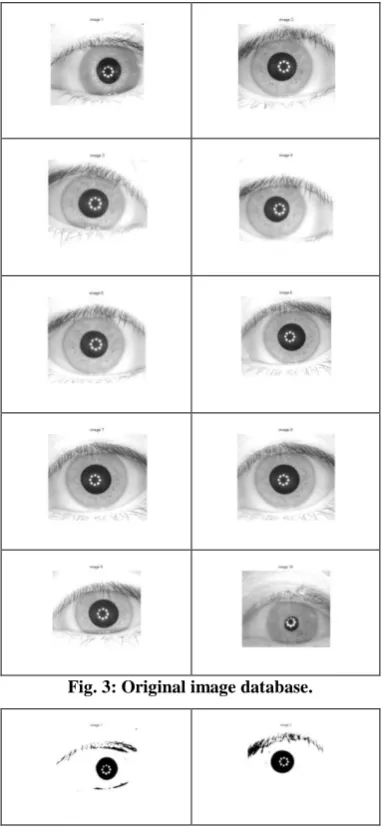
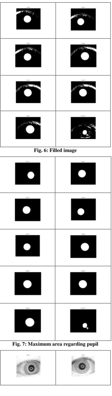
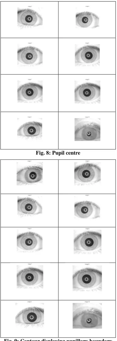
[image:4.595.333.525.324.743.2]

The algorithm is tested over 10 CASIA iris images original database as shown in Fig. 3. The input image is first converted to the binary image as shown in Fig. 4. This is the first step to find the pupillary boundary. After converting to the binary images, the next step is to convert these into their complemented form as shown in Fig. 5 to remove the specular reflections from the images. These specular reflection holes are filled by dilation process as shown in Fig. 6. After removing the specular reflections the maximum area which gives the pupils are shown in Fig. 7. The maximum area regarding the pupil is used to find the centre of pupil as shown in Fig. 8. Fig. 9 displays the pupillary boundary by drawing a circle around the pupillary boundary. Fig. 10 shows the iris boundary which is obtained using daugman’s operator [12].

[image:5.595.333.526.68.750.2]

Fig. 4: Binary image

Fig. 5: Complemented image

Fig. 6: Filled image

[image:5.595.71.263.69.718.2]

[image:6.595.333.525.68.321.2]

Fig. 8: Pupil centre

[image:6.595.71.264.70.628.2]

Fig. 9: Contour displaying pupillary boundary Contour Showing Iris Boundary

Fig. 10: Contour displaying iris boundary

3.2

Result of DRLSE Algorithm

This algorithm is tested over 8 CASIA iris images and step by step observation is shown in the following tables:

3.2.1 Table for Original Images:

This table has the 8 iris images from the CASIA database.

Original Image

[image:6.595.348.508.402.680.2]

Median filtered Image

3.2.3 Table for Initial Contour position Images:

The next step in algorithm is to set the position of contour. This table is showing the initial position of contour with respect to image taken

.

Initial Contour position Images

3.2.4 Table for Contour Images:

This table is showing the path of contour which is moving towards iris edges.

Contour Image

3.2.5 Table for Contour highlighting Iris Images:

This is the result of algorithm. The table shows the resultant image i.e. the final contour highlighting the iris boundary

.

The algorithm is also compared with the algorithm of Hough Transform on the basis of computational time. The proposed algorithm uses 12.056 sec to display the result while the computational time for the Hough Transform is about 248.23 sec. So on the computational time, the implemented algorithm is better than the Hough Transform algorithm.

4.

CONCLUSIONS

Iris localization is the beginning task in any iris-based biometric authentication system and if the iris part of an eye image is not detected accurately then it leads to errors in overall identification method. In this work, two algorithms are studied for iris localization. The first algorithm, Daugman’s operator uses basic integration and differentiation technique to highlight the iris image. The second algorithm DRLSE uses internal energy, external energy concept to localize the iris boundary. From the result of both algorithms, it is concluded that the accuracy of iris localization is depending upon the intensity of iris image. Some images are of dark intensity and some images are of light intensity. The time taken by DRLSE is less then as compared to Daugman’s operator. The accuracy of DRLSE is 98.6% as compared to 96.7% of the Daugman’s operator.

5.

REFERENCES

[1] S. Dey, D. Samanta and J. Daugman, “How iris recognition works,” IEEE Trans on Circuits and Systems for Video Technology, vol. 14, no. 1, pp. 21– 30, 2004.

[2] Inmaculada Tomeo-Reyes, Judith Liu-Jimenez, Ivan Rubio-Polo, Jorge Redondo-Justo and Raul Sanchez-Reillo,” Input images in iris recognition systems: a case study”. IEEE SysCon, pp. 501-505, 2011.

[3] S. Dey, and D. Samanta, , “ Iris data indexing method using Gabor energy features” IEEE Trans on Information Forensics and Security, vol. 7, no. 4, August 2012.

[4] Sarah E. Baker, Amanda Hentz, Kevin W. Bowyer and Patrick J. Flynn, “Degradation of iris recognition performance due to non-cosmetic prescription contact lenses”, computer vision and image understanding, vol. 114, pp. 1030-1044, 2010. .

[5] Zhaofeng He, Tieniu Tan, Zhenan Sun and Xianchao Qiu. “Toward accurate and fast iris segmentation for iris biometrics”, IEEE transactions on pattern analysis and machine intelligence, vol. 31, pp. 1670-1684, 2009.

[6] Rajesh Bodade and Dr. Sanjay Talbar, “Dynamic iris localization: A novel approach suitable for Fake Iris Detection”, IEEE Conference on ultra-modern telecommunication and workshop, pp. 1-5, 2009.

[7] Milos Stojmenovic, Aleksandar Jevremovic and Amiya Nayak, “Fast iris detection via shape based circularity”, IEEE Conference on industrial electronics and applications, pp. 747-752, 2013.

[8] Kaushik Roy, Prabir Bhattacharya and Ching Y. Suen, “Iris segmentation using variational level set method”, Optics and laser in engineering, vol. 49, pp. 578-588, 2011.

[9] Abduljalil Radman, Kasmiran Jumari and Nasharuddin Zainal, “Fast and reliable iris segmentation algorithm”, IEEE transaction on image processing, vol. 7, pp. 42-49, 2013.

[10]R. P. Ramkumar, and Dr. S. Arumugam. “A novel iris recognition algorithm”. IEEE conference on computing communication and networking technologies, pp. 1-6, 2012.

[11]Chung-Chih Tsai, Heng-Yi Lin, Jinshiuh Taur, and Chin-Wang Tao,” Iris Recognition Using Possibilistic Fuzzy Matching on Local Features” IEEE transactions on systems, man, and cybernetics, vol. 42,, 2012.

[12]R.B. Dubey, Abhimanyu Madan, “Iris Localization using Daugman’s Intero-Differential Operator” International Journal of Computer Applications (0975-8887), vol. 93 no. 3, 2014.

[13]V. Caselles, F. Catte, T. Coll, and F. Dibos, “A geometric model for active contours in image processing,” Numer. Math., vol. 66, no. 1, pp.1–31, Dec. 1993.

[14]R. Malladi, J. A. Sethian, and B. C. Vemuri, “Shape modeling with front propagation: A level set approach,” IEEE Trans. Pattern. Anal.Mach. Intell., vol. 17, no. 2, pp. 158–175, Feb. 1995.

[15]J. Sethian, Level Set Methods and Fast Marching Methods. Cambridge, U.K.: Cambridge Univ. Press, 1999.

[16]S. Osher and R. Fedkiw, Level Set Methods and Dynamic Implicit Surfaces. New York: Springer-Verlag, 2002. [17]M. Sussman, P. Smereka, and S. Osher, “A level set

approach for computing solutions to incompressible two-phase flow,” J. Comput. Phys., vol. 114, no. 1, pp. 146– 159, Sep. 1994.

[18]A. Harjoko, S. Hartati, and H. Dwiyasa, “ A Method for Iris Recognition Based on 1D Coiflet Wavelet”, World Academy of Science, Engineering and Technology 56, 2009.

[19]R. T. Al-Zubi and D. I. Abu-Al-Nadi, “Automated personal Identification System Based on Human Iris Analysis”, Pattern Analysis Application, vol. 10: pp. 147–164, 2007.

[20]L. Berggren, “Iridology: A critical review”, ActaOphthalmoligica, vol. 63, pp. 1–8, 1985.