Integration of migrants in Italy: A simple general and objective measure

Munich Personal RePEc Archive

Integration of migrants in Italy: A

simple general and objective measure

Di Bartolomeo, Anna and Di Bartolomeo, Giovanni

April 2007

Online at

https://mpra.ub.uni-muenchen.de/4421/

F

C

Department of Communication, Working Paper No. 10 – 2007

Integration of migrants in Italy: A simple

general

and

objective

measure

Anna Di Bartolomeo

Università di Roma “La Sapienza”

Giovanni Di Bartolomeo

Università degli Studi di Teramo

April, 2007

Abstract. Measuring migrants’ integration into host societies is a challenging task as, in general, measuring any social behavior and social phenomena. The task is affected by many specific problems related to the definition of the objective of study and the impact of subjective evaluations in the construction of an index. Our study aims to provide a measure of integration as much as possible general and objective. More

in details, first, we consider some different general aspects of the

integration problem related to migrants’ polarization, cultural diversification, social stability, integration in the labor market. Second,

we aggregate them in a synthetic linear index, which is rather objective

since the weights are computed by only considering the statistical properties of our dataset, i.e. choosing those weights that minimize the information loss in terms of data variances/co-variances.

1. Introduction

Understanding and monitoring the diversity that lies under migrants’ integration trends

is a challenge that policymakers must be able to face. The challenge is important for

governments and local administrations, but it is not limited to the national borders. The

issue is a general and faced by all European institutions at different levels. In this vein,

migrants’ integration can be placed in the more general issue of social cohesion, one of

the main policy targets of the European Union as the support of technological

innovation in the so-called Lisbon Strategy.

The migrants’ integration is also a challenging issue for its multi-disciplinary nature and

extended implications. Migrants’ integration is a socio-economic process that needs to

be understood of expertise that varies from psychology to law or geo-political

knowledge. Moreover, the growing impact of migrants on population affects other

policy debate from the reform of social security to the education system organization.

Political and socio-economic scientists as well as policymakers, in their current

activities, need quantitative data to evaluate the impact of policy and to understand and

monitor the current situation.

This paper attempts to derive a general index of integration. The aim of our index is to

give a general picture of integration reached and, in particular, of the differences among

Italian regions. The index is, of course, complementary to other indicators1 (as

specifically those related to specific micro-context) and not exhaustive of the

phenomenon because of the variety and extent of the migrants’ integration phenomenon.

The issue of measuring the integration of migrants into host societies is a challenging

task as, more in general, quantifying any social behavior and social phenomena. In

particular, measuring integration means evaluating two social processes since one

cannot look at the migrants alone, but also has to take the members of the host society

into consideration (see Borjas, 1994, 1999, Bauer and Zimmermann, 1997).2

The cornerstone for a measure of integration is its own definition since the concept of

what integration means and is to achieve differs. These differences are reflected in the

1

Other indicators will be later presented. 2

An interesting specific aspect is that of the sentiments of natives towards immigrants. See, e.g. Bauer et al. (2000), who explore the possibility that immigration policy may affect the labor market assimilation of immigrants and natives’ sentiments towards immigrants.

national policy goals and range from next-to-assimilation to multiculturalism. Different

definitions of what integration means form the basis of the national policies for

improving migrants' integration, the standard of when integration can be considered

successful varies.

This is important when it comes to compare the integration of migrants in different

countries and societies: It is because of these differences that the principal concepts of

integration and the different national policies resulting from these concepts need to be

looked at more closely, because they form the background for evaluating migrants’

integration. The national policies often reflect different definitions of what is meant by

integration. Although the term itself means joining parts (in) to an entity, its practical

interpretation and social connotation may vary considerably: Assimilation as well as

multicultural society may be considered synonyms or descriptions of (successful) integration. Thus, all forms of cultural or social behavior ranging from completely

giving up one’s background to preserving unaltered patterns of behavior are covered by

the term of integration. This problem of definition, of course, has a bearing on

measuring integration, because the requirements for success in assimilation are much

more difficult to meet than requirements for multicultural coexistence in a society that

remains indifferent about other people’s rites or customs.

Notwithstanding the definition or concept of integration applied, one will agree that the

integration of migrants into their respective host societies has at least four basic

dimensions concerning the social, economic and cultural (in terms of both assimilation

of the host society culture and of the native culture) role migrants play in their new

environment. We can summarize integration in four dimensions:

1) the degree of polarization,

2) cultural diversification,

3) social stability,

4) integration in the labor market.

These four dimensions will hardly be disputed by anybody as important fields of

integration. See, among others, Borjas (1994), Freeman (1995), Hansen (1999), Rogers

Penninx (2004), Geddes and Niessen (2005), which deeply discuss and survey different

integration aspects.

This paper considers the above dimensions of interaction and by taking account of them

provides an aggregate measure of integration. The task of measuring integration is

affected by many specific problems related to the definition of the objective of study

and the impact of subjective evaluations in the construction of the index, these aspects

cannot be neglected. This paper aims to provide a measure of integration as much as

possible general and objective. We consider the aforementioned aspects of integration

and aggregate them in a synthetic one-dimensional index by using the principal

component analysis. Our index is computed at a regional level; thus, it ranks region

levels of integration.

There are some related studies to our paper. The first is a CNEL study of 2004 (CNEL,

2004). This study investigates the regional differences by considering the four

dimensions above described. It aggregates twenty indicators by a simple ordinal

procedure. We will describe it more in detail in the next sections since our dataset is

based on this study. Another attempt to measure general integration is provided by the

Italian Commission for integration policy,3 which proposed the concept of “reasonable

integration” founded on no discrimination and of inclusion of differences. This concept

can be related to two dimensions of integration: integrity of the individual and positive

integration. The former means well-being and the latter living together peacefully (see

Zincone, 2000, 2001).

All aforementioned studies are inspired by the Council of Europe guidelines in terms of

social cohesion (Council of Europe, 2000) and are in line with the European debate on

migrants’ integration. In 2003, the European Commission has underlined the priorities

and political orientations on the consolidation of a legal European structure on

immigration, the strengthening of coordination policies, the attention towards processes

of integration and social inclusion, including attempts to have detailed and statistically

homogeneous information on the evolvement of the migratory fluxes.4 The OECD also

3

See Golini et al. (2001). 4

See the European Commission Report on immigration, integration and employment, 2003. See also the

First report on integration and immigration in Europe (2004), the Handbook on integration (2005), the

stress that to be effective, integration actions need to be based on the gathering and

analysis of information (see OECD, 2006)

The studies of the CNEL and Commission for integration policy attempt to give the

general picture of the integration in Italy. However, it should be note that specific

indexes are as much important since migrants’ integration has a specific nature that

varies according to the different dimensions under scrutiny or a geographical diminution

that can have a high degree of heterogeneity. Although we do not survey these indexes5

here because we also aim to build a general index, we would like to underline that the

policymaker needs of both to coordinate their decisions at a micro and macro levels.

Geddes and Niessen (2005) develop the “European civic citizenship and inclusion

index,” which is an attempt to measure the potential effectiveness of the actions

implemented by several member states as “civic citizenship” policies and for the job

market. The index is not related to the success of the immigrants’ integration process,

but it measures if the legal conditions to support such a goal have been created. The

inclusion indicators were chosen for each of the five legal fields that seemed to be more

relevant for integration: 1) labor market, 2) residence, 2) family reunion, 4)

naturalization, 5) addressing discrimination.

The rest of the paper is structured as follows. Section 2 describes our dataset, which is

collected by CNEL (2004). Section 3 compares our aggregation methodology to that

used in CNEL (2004). Section 4 derives and comments our result. A final section

occludes our work.

2. Integration and our data

At the beginning of 2004, according to the data of the Ministry of Interior Affairs,

regular migrants in Italy were 2.2 millions. The data of the Ministry is the most relevant

for policy analysis and refers to the people who have requested a residence permit. This

data underestimates migrants since it does not takes account of the migrants under 18

years. Each year, the data is corrected by the CARITAS report on migration; in 2004

migrants are estimated as 2.6 millions. Migrants thus represents about 4.5% of the

5

Italian population (one migrant each 22 residents) and by considering the net flow,

which is 681.665 units, their number is increased of 45% between 2003 and 2004 (cf.

CARITAS, 2004). Migrants are also reordered by ISTAT, which consider the census

data. The unit of observation of the census data is the resident migrants, who are

migrants registered at the General Registry Office a sub-sample of migrants who have

requested the residence permit (registered by the Ministry for Interior Affairs). The first

of January 2004, the resident migrants were 1.990.159 (978.232 female and 1.011.927

male). The resident migrants were thus the 3.4% of the total number of residents with an

increase with respect to the previous year of 28.4%.

All the data register the growing relevance of the migrants’ dimension and thus of the

associated problems and perspectives. Migrants have a heterogeneous composition and

distribution in the territory. Their incidence is stronger in the Northern and Central

regions. The most represented foreign nationalities are Rumania, Morocco and Albania,

followed by Ukraine and China. However, migrants are uneven distributed since they

tens to concentrates according to their nationality; an emblematic case is that of the

Chinese in the province of Prato, who represent almost the 100% of the migrants and

more than the 50% of the population.

Italy becomes a country of immigration in the 1970s from a long experience of

emigration. Although it is a country that only recently experienced this phenomenon, it

has already face the evolution of the immigration process from the first to the second

generations and a growing number of new problem related to the integration. The

change from the emigration to the immigration perspective and the economic impact of

the immigration are described in details by Del Boca and Venturini (2005).

In 30 years, integration thus becomes a very lively debated issue as well as the policies

supporting it important in both the domestic and the European,6 the problem of

international is, in fact, related to the more general discussion on the European welfare

system (see Boeri et al. 2002). The debate is complex and articulated. The common

departing point should be however that of measuring integration both for positive and

normative analysis. Integration can be measured by different factors that can be grouped

in subjective and objective measures. After a long preliminary study, CNEL (2004) has

6

summarized information about integration in some indicators, which represents our

dataset.7 It collects a group of indicators that represent the migrants’ integration under

different perspectives. More in details, CNEL individuates twenty key indicators, which

are describes below.

1. Incidence (INC) measures the quota of foreign residents on the total number of

residents in each region.

2. Incremental indicator (INR) measures the percent variation of foreign residents

between 1992 and 2002.

3. Permanence (PER) is the proportion of net migrant flows (residence permits

released in the year and still valid at the end of the year) on the gross flows

(residence permits released in the year).

4. Flow indicator (FLU) is the incidence of the new net flow of migrants on the

total amount of resident foreigners.

5. Pluralism indicator (PLU) is the number of foreign nationalities represented by

foreign resident in each region.

6. National heterogeneity 1 (ET1) measures the incidence of the largest foreign

national group on the total amount of foreign residents.

7. National heterogeneity 2 (ET2) measure the incidence of the ten foreign groups

more present on the total number of migrants.

8. Continental heterogeneity (ETC) is the degree of diversification of the

continental representatives, which is computed among the 10 foreign groups

more numerous within the migrants, It is build by an index number that

considers the migrants’ continental areas, the number of migrants’ ethnic groups

of the continent more represented (for more details, see CNEL, 2004).8

9. Religious difference (REL) measures the heterogeneity of the regional

confessions among migrants. It is the number of people accepting the more

diffused religious confession on the number of migrants.

7

The dataset is presented in the appendix (see Table 1.A). 8

10.Family reunion (RIC) is the incidence of foreign resident for family reasons on

the total amount of them.

11.Long (LUN) measures the long stays, i.e. the incidence of migrants who are

present from at least 10 years on the total number of migrants in 2000.

12.Citizenship (CIT) is the yearly number of foreign resident who acquire the

Italian citizenship for every 1.000 foreign residents.

13.Stability residence (STA) indicates the incidence of stable residents on the total;

stable residents are people resident for job, adoption, rejoining, study, religion,

elective residence, waiting for citizenship.

14.Deviance (DEV) is the incidence of resident foreigners complained to the police

authorities on the total number of resident foreigners (2001).

15.Potential employment (OCP) is the incidence of the foreign labor force on total

of foreign residents.

16.Effective employment (OCE) is the percentage of the foreign unemployed on the

foreign labor force.

17.Labor market sustainability (LAV) corresponds to the migrants’ incidence of the

net yearly flow of migrants hiring on the total number of net hiring;

18.Entrepreneurship (IMP) is the proportion of foreign entrepreneurs on the total

number of foreign citizens.

19.Work injury (INF) is the percentage of indemnities paid to foreign citizens on the

total indemnities in 2001.

The above indicators can be grouped according to the integration dimension they

capture. More in details, PER, INC, PRE, INR, FLU can be related to the degree of

polarization; ET1, ET2, ETC, REL, LUN can be associated to the cultural

diversification; STA, RIC, DEV, PLU, CIT concern about the social stability; and LAV,

OCE, OCP, INF and IMP summarize the integration in the labor market. In the next

section we critically describe how these indicators are aggregated by the CNEL study

Finally note that, as it will be later clear, to perform our analysis it is convenient to

consider quantitative indicators that display a value of zero for the lower possible level

of integration. Thus, our indicators are slightly different from the original data of

CNEL. We transformed some original data to obtain positive (increasing) measures of

integration and a zero measure for no integration. More in detail, we considered the

complement to one of the following indicators: ET1, ET2, DEV, OCE, INF and REL,

which in the original dataset are negative (decreasing) measures of integration. In our

framework, the interpretation of the indicators is exactly opposite to the original one

and the transformation is without any loss of generality since all variables were

expressed in percentage terms. For instance, consider OCE, in the original data set it

indicates the incidence of the unemployed on the total labor force within migrants; a

high value measures a low integration. By contrast, in our setup OCE indicates the

complement to one of the original variable, i.e. the incidence of the employed on the

total labor force within migrants and high values of OCE measure a high integration.

3. The CNEL aggregation and our methodology

The CNEL index is obtained by a two-step aggregation procedure. First all the

indicators are transformed in ordinal variables. Each of the 20 indicators is ordered and

a number between 1 and 20 assigned, 20 is also the number of observations i.e. the

Italian regions, 20 (1) for the highest (lowest) score, which indicates the best (worst)

performance in terms of integration. At the end each region is thus classified on the

basis of its ordinal rank.9 Second, transformed indicators are aggregated by simple sum

of the region scores. There are two levels of aggregation. The first one is partial and

measures the integration under the different aforementioned four dimensions of the

integration by considering only the indicators that refer to a specific dimensions (i.e.

polarization; cultural diversification; social stability; integration in the labor market);

the second measures the general level of integration and takes account of all of them.

For instance, after the dataset transformation in ordinary values, by summing the scores

of Abruzzo in PER, INC, PRE and INR, we obtain the value for the index of

9

polarization for Abruzzo, by summing all the indicators we derive the score of CNEL

integration index for Abruzzo.

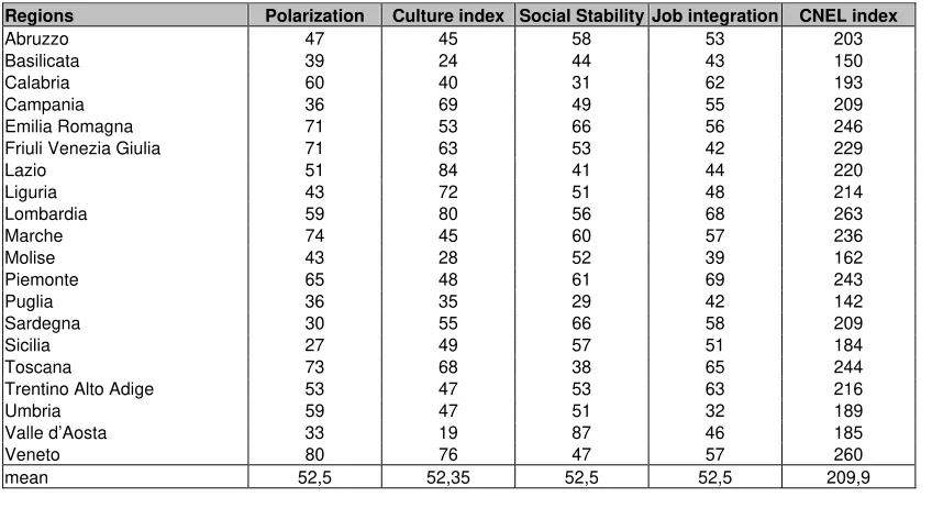
The four sub-indexes and the CNEL integration index obtained as described above are

reported in the following table.

Table 2 – The CNEL indexes.

Regions Polarization Culture index Social Stability Job integration CNEL index

Abruzzo 47 45 58 53 203

Basilicata 39 24 44 43 150

Calabria 60 40 31 62 193

Campania 36 69 49 55 209

Emilia Romagna 71 53 66 56 246

Friuli Venezia Giulia 71 63 53 42 229

Lazio 51 84 41 44 220

Liguria 43 72 51 48 214

Lombardia 59 80 56 68 263

Marche 74 45 60 57 236

Molise 43 28 52 39 162

Piemonte 65 48 61 69 243

Puglia 36 35 29 42 142

Sardegna 30 55 66 58 209

Sicilia 27 49 57 51 184

Toscana 73 68 38 65 244

Trentino Alto Adige 53 47 53 63 216

Umbria 59 47 51 32 189

Valle d’Aosta 33 19 87 46 185

Veneto 80 76 47 57 260

mean 52,5 52,35 52,5 52,5 209,9

Source: CNEL (2004).

According to the CNEL results, Italy is divided in three areas of integration. Above the

average: Lombardia, Veneto, Emilia Romagna, Toscana, Piemonte, Marche and Friuli

Venezia Giulia, respectively; close to the average: Lazio, Trentino Alto Adige, Liguria,

Campania, Sardegna, Abruzzo and Calabria; below the average: Umbria, Valle d’Aosta,

Sicilia, Molise, Basilicata and Puglia. The index emphasizes regional heterogeneities

and an easier integration in the North of the country. Regions also display certain

heterogeneity.

The procedure followed by CNEL to build the index has two main limitations:

1. It does not consider the relative distance among regions (by assuming an ordinal

score to the region according to their absolute position);

2. It attributes the same weight (1/20) to all variables in the construction of the

Our aim is to obtain an index that takes account of the above criticisms by using an

alternative procedure of aggregation. We directly aggregate the 20 indicators described

in Section 2 without transforming them by the principal component analysis.

Principal components analysis is one of the best-known and earliest ordination methods,

first described by Karl Pearson (1901). The underlying idea is to reduce the

dimensionality of the dataset by retaining its variability as much as possible and derive

synthetic indices of integration. Formally, it consists of an eigen-analysis of a

covariance or correlation matrix calculated on the original measurement data.

The principal component analysis searches for a few uncorrelated linear combinations

(principal components) of the original variables that capture most of the information in

the original variables.10 In the bi-dimensional case, one can summarize the correlation

between two variables by a scatter plot and a regression line. The regression line

represents the best summary of the linear relationship between the variables. If we could

define a variable that would approximate the regression line, that variable would capture

most of the essence of the two original variables, i.e. the dataset. The subjects’ single

scores on that new factor, represented by the regression line, could then be used in

future data analyses to represent that essence of the two items. In a sense, we have

rebuilt the two variables to one factor or component – the factor is in fact a vector made up of two numbers that can be conceived as weights on the former variables. Note that

the new factor is actually a linear combination of the two variables and its significance

increases in the two-variable correlation.

The example described above, which combines two correlated variables into one factor,

illustrates the basic idea of principal components analysis. If we extend the two-variable

example to multiple variables, then the computations become more involved, but the

basic principle of expressing two or more variables by a single factor remains the same.

By considering more than two variables, we can think of them as defining a space, just

as two variables defined a plane. Thus, when we have three variables, we could plot a

10

three-dimensional scatter plot, and, again we could fit a plane through the data (a plane

will individuate by two orthogonal lines). In the principal components analysis, after the

first factor has been extracted, that is, after the first line has been drawn from the data,

we continue and define another line that best fits the remaining variability, and so on. In

this manner, consecutive factors are extracted.

The principal component analysis can be performed by considering centered and non-

centered data. In the latter original data are used. In the former entries of the matrix of

data are transformed in deviations from the mean of the variables. The difference

between the two procedures is however not trivial and we need to discuss it as it is

relevant for our investigation. Non-centered principal components analysis implies an

all-zero point (vector) of reference: no interlock linkages. By contrast, centering on, or

normalizing by, some variables shifts the reference points to a hypothetical average

stand.11 Our benchmark is the case of no integration and we are attempting to find a

measure of how much each region differs from this reference point, we thus consider

the non-centered analysis, i.e. the zero vector as benchmark i.e. no integration.12

4. Empirical results

The principal component analysis produces a synthetic picture of a dataset by reducing

the loss of information, i.e. in term of explained variance. The principal component

analysis extracts, from the data matrix, the linear weights (loading) used to build an

index (component) from the data. One the first component is extracted, the process is

replicated and a second one obtained. The second component is the set of weights that

minimize the explained variance under the additional constraint of obtaining a

component uncorrelated to the first one. The process can be replicated as the number of

components is equal to the number of variables and all the expected variance is

replicated.

The principal component analysis can be performed by using either the mean deviations

(centered analysis) or not (non-centered analysis). The former synthesizes the sample

variability with respect to a hypothetical average observation (region, in our case). The

11

See Di Bartolomeo and Marchetti (2003) or Carbonai and Di Bartolomeo (2006) for discussions about the two procedures for some specific cases. See Noy-Meir (1973) for a general discussion.

12

latter investigates the variability with respect to an hypothetical region scoring zero to

all observed variables, which correspond to a region with the minimum degree of

integration. Moreover, the principal component analysis can be performed by

considering either the standardized or the non-standardized variables. The best

methodological choice depends on the researcher’s aim and the problem under scrutiny.

We consider standardized variables in a non-cantered analysis. We standardize the

variables to eliminate the effects of the unit of measure since not all the variables are

expressed in terms of ratio and as already claimed we use the non-centered analysis

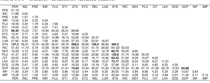
since our benchmark is the worst case of no integration.

Table 3.A – Dataset variance/covariance matrix.

PER INC PRE INR FLU ET1 ET2 ETC REL LUN STA RIC DEV PLU CIT LAV OCE OCP INF IMP PER 51,19

INC 11,88 3,64

PRE 5,94 1,57 1,76

INR 13,53 3,34 2,33 4,54

FLU 18,59 4,30 1,79 4,39 7,68

ET1 19,02 4,41 1,85 4,47 7,41 8,34

ET2 66,40 15,22 7,51 16,99 24,52 26,01 88,86

ETC 12,47 2,77 1,76 3,01 4,65 5,21 16,99 4,25

REL 40,19 9,52 4,85 10,42 14,98 16,15 53,65 10,54 33,37

LUN 27,95 6,03 3,64 7,55 9,90 10,44 37,23 7,26 22,61 16,87

STA 157,2 36,21 19,70 42,28 56,61 59,76 208,0 39,66 126,0 88,60 494,2

RIC 51,43 11,74 5,79 12,99 18,90 19,93 68,50 13,01 41,14 28,63 161,02 53,53

DEV 19,59 4,15 2,02 4,57 7,68 7,76 25,96 5,25 15,77 10,79 60,75 20,20 8,60

PLU 41,37 9,57 5,80 11,66 14,58 15,20 53,99 10,60 32,82 23,30 129,8 41,74 15,66 35,03 CIT 20,02 4,52 1,88 4,68 7,85 8,02 26,80 4,89 16,17 10,94 62,32 21,02 8,39 15,67 8,92 LAV 23,41 5,44 3,03 6,30 8,52 8,97 31,00 6,17 18,89 13,27 73,17 23,65 9,24 19,36 9,07 11,91

OCE 12,29 2,47 1,32 2,92 4,92 4,97 16,35 3,53 10,18 7,22 37,69 12,37 5,11 9,93 4,82 6,22 4,00 OCP 56,64 13,43 7,52 15,70 20,07 21,41 74,83 14,34 45,61 31,94 178,24 57,54 21,46 47,15 21,90 26,76 13,53 64,98

INF 11,85 3,24 1,78 3,80 3,92 3,96 15,03 2,44 9,05 6,25 36,55 11,55 3,84 9,86 4,22 5,35 2,28 13,67 3,64 IMP 10,29 2,47 1,30 2,51 4,09 3,87 13,58 2,84 8,33 6,12 32,04 10,61 4,09 8,65 4,16 4,86 2,91 11,40 2,11 3,14

PER INC PRE INR FLU ET1 ET2 ETC REL LUN STA RIC DEV PLU CIT LAV OCE OCP INF IMP

By using the above matrix, we obtain the loadings indicated in Table 2 for the first

component as result of a non-centered principal component analysis on standardized

data.

Table 2 – First component loadings.

Indicators (1/2) Loadings (1/2) Indicators (2/2) Loadings (2/2)

The first component explains the 99% of sample variance; we thus do not consider the

other components, which are reported in the appendix. The indicators that contribute

more to the index are emphasized.

The region scores are reported in the following table that also indicates the average

deviation from the average region.

Table 2 – Integration index.

Regions Integration index Average % deviation

Marche 13,018 3,04%

Friuli Venezia Giulia 12,881 1,95%

Lombardia 12,874 1,90%

Trentino Alto Adige 12,874 1,90%

Piemonte 12,854 1,74%

Veneto 12,841 1,64%

Lazio 12,830 1,55%

Umbria 12,827 1,52%

Emilia Romagna 12,760 0,99%

Abruzzo 12,736 0,80%

Sardegna 12,730 0,76%

Valle d’Aosta 12,695 0,48%

Toscana 12,626 -0,07%

Sicilia 12,590 -0,35%

Campania 12,489 -1,15%

Puglia 12,377 -2,04%

Liguria 12,369 -2,10%

Molise 12,326 -2,44%

Basilicata 12,235 -3,16%

Calabria 11,756 -6,95%

Mean 12,634 0.00%

The table describes the index (left column) and the percentage deviation of each region

with respect to the Italian regional average (right column). Marche, Friuli Venezia

Giulia, Lombardia are above the average. Emilia Romagna, Abruzzo, Sardegna, Val

d’Aosta, Toscana and Sicilia are closet o the average. Campania, Puglia, Liguria,

Molise, Basilicata and Calabria are below the average. Marche achieves the best

performance (3,04% above the average), Calabria the worst one placing itself largely

below the average (-6,95%). The index displays great and net heterogeneity in favor of

the North Regions.

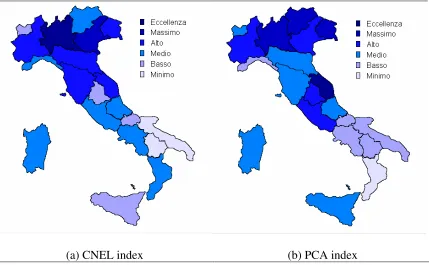
Figure 1 – A comparison between the CNEL index and our index.

(a) CNEL index (b) PCA index

According to our index, the most integrated region is Marche, instead of Lombardia

(CNEL index), which is one of the most integrated regions, but it occupies only the

third position in PCA index. The distance between the North and the South of Italy is

magnified, whereas the performance of the central Italy is greatly improved.

5. Conclusions

Measuring migrants’ integration into host societies is a challenging task sine the many

specific problems related to the definition of the objective of study and the impact of

subjective evaluations in the construction of an index cannot be neglected. In this study,

we have provided a measure of migrants’ integration relatively general and objective.

We have considered some important aspects of integration by taking account of 20

indicators, derived from a preliminary CNEL study that have derived these indicators

from a more large set. The 20 indicators measure different general aspects of migrants’

integration about polarization, cultural diversification, social stability, integration in the

labor market at a regional level. Then we have aggregated these indicators in a linear

computed by only considering the statistical properties of the dataset. In other words,

weights have been chosen by minimizing the dataset information loss.

Our study shows a further element of division between the North and South of Italy,

which is alarming news and a public policy field since the growing relevance of the

immigration problem. We have in fact found that Italy can be divided in some different

macro regions with very different levels of integration. In particular, by comparing our

results to those of previous studies, we found that there is not a substantial difference

between the North and Centre Italy, many central regions performs better than those of

the North. In contrast, the difference between North and South Italy is more than that

previously documented. The performance of the Sicily and Sardinia is more close to

that of the regions at the bottom of the North Italy that to that of the southern regions.

Acknowledgments

We are grateful to Antonella Guarnieri for her comments on previous versions.

References

Bauer, T. and K.F. Zimmermann (1997), 'Integrating the East: The labor market effects

of immigration,' in: S.W. Black (ed.), Europe’s economy looks East - Implications for

Germany and the European Union, Cambridge, Cambridge University Press, 269-306. Bauer, T., M. Lofstrom and K.F. Zimmermann (2000), “Immigration policy, assimilation of immigrants and natives’ sentiments towards immigrants: Evidence from

12 OECD countries,” Swedish Economic Policy Review, 7: 11-53.

Billotta, E, A. Di Bartolomeo, A. Guarneri, M. Simone (2006), “Opinioni e atteggiamenti degli studenti: un’indagine nelle scuole medie del Lazio”, Proceedings of

the Conference on Giornata studio sull’integrazione dei minori immigrati nelle scuole

at the University of Rome La Sapienza.

Boeri, T., G. Hanson and B. McCormick (2002), Immigration policy and the welfare

system, Oxford University Press, Oxford.

Borjas, G.J. (1994), “The economics of immigration,” Journal of Economic Literature,

32: 1667-1717.

Borjas, G. J. (1999), “The economic analysis of immigration,” in O. Ashenfelter and D.

Card (editors), Handbook of Labor Economics, Vol. 3A, New York, North Holland.

CNEL (2004), “Immigrazione in Italia. Indici di inserimento territoriale. III Rapporto,” CNEL, Roma.

Del Boca D. and A. Venturini (2005), “Italian migration,” in Zimmermann (2005): 303-336.

Di Bartolomeo, G. and E. Marchetti (2004), “Central banks and information provided to

the private sector,” BNL Quarterly Review, 230: 265-297.

Entzinger H. and Biezveld R. (2003), Benchmarking on immigrant integration, report

for the European Commission by European Research Centre on Migration and Ethnic

Relations (ERCOMER), EU project No. DG JAI-A-2/2002/006.

Freeman, G. (1995), “Modes of immigration politics in liberal democratic states.”

International Migration Review 29: 881-902.

Geddes A. and J. Niessen (edotors) (2005), European civic citizenship and inclusion

index, Foreign Policy Center, Migration Policy Group, British Council Brussels, Brussels.

Golini A., S. Strozza, F. Amato (2001), “Un sistema di indicatori di integrazione: primo tentativo di costruzione,” in Zincone (2001).

Gregori E. and L. Mauri (2005), “Un paniere di indicatori per il monitoraggio

dell’integrazione sociolavorativa degli immigrati” in Dinamiche di integrazione

sociolavorativa di immigrati. Ricerche empiriche in alcuni segmenti del mercato del lavoro lombardo edited by Cologna D., E. Gregori, C. Lainati, L. Mauri, Synergia, Guerini e Associati, Milan.

Gregori, E. (2006), “Indicators of migrants’ socio-professional integration,” FEEM Nota di Lavoro No 59.

Hansen, R. (1999), “Migration, citizenship and race in Europe: Between incorporation

and exclusion,” European Journal of Political Research 35: 415-444.

Jolliffe, I.T. (1986), Principal components analysis. Springer-Verlag, Berlin.

Noy-Meir, I. (1973), “Data transformation in ecological ordination: I. Some advantage

of non-centering,” Journal of Ecology, 61: 329-341.

OECD (2006), From immigration to integration: Local solutions to a global challenge,

OECD, Paris.

Penninx, R., K. Kraal, M. Martiniello and S. Vertovec (2004), Citizenship in European

Cities: Immigrants, Local Politics and Integration Policies. Aldershot, Ashgate.

Rogers A. and J. Tillie (2001), Multicultural policies and modes of citizenship in

European cities. Aldershot, Ashgate.

Zincone, G. (editor) (2000), Primo rapporto sull’integrazione degli immigratiin Italia,

Commissione per le politiche di integrazione degli immigrati, Il Mulino, Bologna.

Zincone, G. (editor) (2001), Secondo rapporto sull’integrazione degli immigrati in

Italia, Commissione per le politiche di integrazione degli immigrati, Il Mulino, Bologna.

Zimmermann K.F. (2005), European migration: What do we know?, Oxford University

Appendix A – The data set

Table 1.A – CNEL data.

Region PER INC PRE INR FLU PLU ET1 ET2 ETC REL LUN STA RIC CIT DEV OCP OCE LAV IMP INF ABR 38 64,1 1,4 2,8 12,3 142 21,6 65,9 6 35,2 16,9 96,2 42,7 12,4 8,7 46,4 2,9 13 5,2 7,11 BAS 34,9 82,2 0,23 1,05 15 99 32,4 76,3 16 51,2 18,1 93,7 37,1 12 13,1 48,8 7 21,1 0,3 3,2 CAL 41,1 84,8 1,2 1,8 24,8 135 27,7 65 17 50,9 25,5 78,3 28,8 7,56 11,1 42,9 18,8 26,2 11,3 1,9 CAM 36,2 2,1 3,9 2,2 7,2 153 17,5 66,5 14 28,7 27,3 94,5 40,7 4,4 7,6 47,8 9,7 24,1 3,8 2,1 EMI 40,8 110 10 6 9,7 166 17,7 61,3 2 48,7 27,7 97,7 31,8 5,8 5,1 60,2 4,51 14,8 4,92 13 FRI 42,9 75,6 3,2 5,2 13 155 13,1 67,9 6 29,2 22 93,4 36,2 7,7 6,16 47,9 4,1 15,5 3,4 15 LAZ 36 4,3 15,8 7,8 6,7 183 9,9 49 11 36,9 33,4 96,1 22,8 4,45 6,23 49,5 6,9 15,5 2,7 5,1 LIG 40,4 19,5 2,4 3,9 9,8 150 13,3 53,4 9 34,9 28,5 96,8 31,6 9 14,2 50,2 7,3 21,5 2,6 4,4 LOM 25,3 108 23 6,5 7,15 174 11,7 53,6 15 39,8 26,1 97,9 30,4 4,7 5,4 61 4,29 21,7 4,86 11,3 MAR 47,1 204 3,1 4,9 11,2 145 18 61,8 4 43,8 18,2 97,5 36,4 7,61 6 52,8 2,6 17,2 2,97 11,4 MOL 40,9 46,9 0,16 1,2 21,8 91 22,2 70,3 5 38,5 20,8 92,1 41,3 13,9 12,4 38,3 5,1 9,8 3,03 3 PIE 38,3 117 7,1 4,4 10,3 165 22,9 67,7 13 44,2 23,6 97,5 34,1 7,64 6,6 57,3 6,1 22,1 6,5 6,7 PUG 29,3 63,1 2,1 1,3 12,5 141 40,2 67,4 19 51,7 14,5 91,3 33,9 7 8,8 48,5 4,52 12,5 1,9 2,8 SAR 29,4 63,5 0,8 1,06 11,6 131 16,1 62,1 10 35,8 33,6 94,5 37,5 9,5 7,7 40,4 4,26 7,5 12 1,8 SIC 35,5 -23,5 3,3 1,7 7,1 148 19,1 74,6 20 43,3 36,8 95,8 35,8 5,7 7,5 53,7 8 14 3,9 3,1 TOS 41,3 90,4 7,4 5,3 11,2 164 18,2 62,1 12 33,2 21,5 96,7 31 6,4 9,1 51,8 4,28 19,1 5,3 6,5 TRE 34,4 95,2 2,6 5,6 10,1 144 14,3 69 1 34,1 25,4 97,6 27,8 5,5 5,2 62 3,2 23,4 2,1 13,3 UMB 39,1 66,9 2 6,2 11,5 150 20,1 61,6 3 39 19,6 96,9 32,2 5,2 4,1 52,1 5,5 9,2 0,7 10,5 VAS 35,7 67 0,19 3,5 8,2 91 30,4 73,6 8 50,3 35,1 97,8 36,5 8,9 4,8 53,8 8,2 20,7 2,8 7,14 VEN 46,1 154 10,2 5,5 10,3 162 15,2 60,9 18 38,8 20,4 97 33,4 5,1 6,1 58,8 3,5 14,8 4,4 14 Mean 37,6 74,8 5,0 3,9 11,6 144 20,1 64,5 10,5 40,4 24,8 95,0 34,1 7,5 7,8 51,2 6,0 17,2 4,2 7,2

Table 2.A – Ranking of the regions.

Table 3.A – PCA results

Axis 1 Axis 2 Axis 3 Axis 4 Axis 5 Axis 6 Eigenvalues 3194.2 5.527 1.759 1.432 1.263 1.192 Percentage 99.431 0.172 0.055 0.045 0.039 0.037 Cumulative Percentage 99.431 99.603 99.658 99.702 99.74 99.78 PCA variable loadings

Axis 1 Axis 2 Axis 3 Axis 4 Axis 5 Axis 6

PER 0.125 0.08 -0.186 0.012 0.005 -0.078

INC 0.026 0.054 -0.596 -0.079 0.027 -0.031

PRE 0.016 -0.335 -0.035 -0.037 0.098 0.144

INR 0.034 -0.298 -0.363 -0.096 0.096 0.121

FLU 0.045 0.321 -0.038 0.141 -0.102 -0.158

ETC 0.032 0.055 0.393 0.128 0.001 -0.033

LUN 0.071 -0.116 0.526 0.107 0.028 0.031

STA 0.393 0.030 0.010 -0.148 0.128 -0.142

RIC 0.128 0.367 -0.004 -0.084 0.197 -0.206

PLU 0.103 -0.295 0.010 0.027 -0.119 0.098

CIT 0.050 0.367 0.009 -0.099 -0.12 -0.181

LAV 0.058 -0.112 -0.027 0.460 0.653 0.033

OCP 0.142 -0.243 0.010 0.066 0.117 0.065

IMP 0.026 0.085 -0.204 0.825 -0.309 -0.046

ET1 0.191 -0.129 0.024 0.000 -0.329 -0.008

ET2 0.092 -0.233 0.000 0.000 -0.491 0.074

DEV 0.577 -0.070 0.000 0.000 0.000 -0.149

OCE 0.477 -0.059 0.000 0.001 0.000 -0.126

INF 0.372 0.348 -0.001 -0.002 0.000 0.769

REL 0.149 -0.181 0.000 0.000 0.005 -0.428

PCA case scores

Axis 1 Axis 2 Axis 3 Axis 4 Axis 5 Axis 6 Abruzzo 12,736 0.479 -0.153 -0.140 -0.117 -0.318 Valle Aosta 12,695 0.381 0.235 -0.052 0.479 0.171 Basilicata 12,235 0.857 0.120 -0.168 0.456 0.185 Calabria 11,756 0.592 -0.014 0.913 -0.119 0.445 Campania 12,489 -0.183 0.379 0.150 0.274 -0.346 Emilia Romagna 12,760 -0.519 -0.272 -0.055 -0.074 -0.098 Friuli Venezia Giulia 12,881 0.028 -0.193 -0.118 -0.061 -0.143

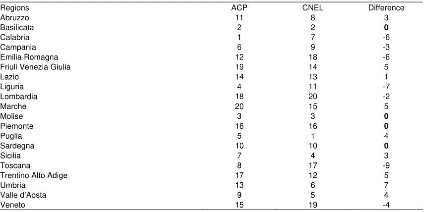
Table 2.B – Index comparison.

Regions ACP CNEL Difference

Abruzzo 11 8 3

Basilicata 2 2 0

Calabria 1 7 -6

Campania 6 9 -3

Emilia Romagna 12 18 -6

Friuli Venezia Giulia 19 14 5

Lazio 14 13 1

Liguria 4 11 -7

Lombardia 18 20 -2

Marche 20 15 5

Molise 3 3 0

Piemonte 16 16 0

Puglia 5 1 4

Sardegna 10 10 0

Sicilia 7 4 3

Toscana 8 17 -9

Trentino Alto Adige 17 12 5

Umbria 13 6 7

Valle d’Aosta 9 5 4