Modelling dependency in multivariate paired comparisons:a log linear approach

attribute

α

comparison (23) comparison

(13)

comparison (12)

θ2.13|α₁ θ1.23|α₁

θ3.12|α₁

attribute

α

comparison (23)

comparison (13) comparison

(12)

θ2.13|α₂ θ1.23|α₂

θ3.12|α₂ β13|α₁α₂

β12|α₁α₂

β23|α1α₂

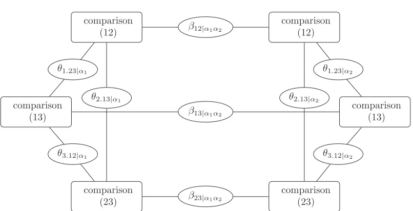
Figure 1: Dependency structure

0 0

.1 0.2 0.3 0.4 0.5 0.6 0

0 .1 0

.2 0

.3 0

.4 0

.5

Green

Conservative

Social democrat Freedom

party

competence in social issues

co

m

p

et

en

ce

in

ec

o

n

o

m

ic

is

su

es

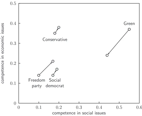
Figure 2: Ascribed competence in social and economic issues

Modelling Dependency in Multivariate Paired

Comparisons: a Log-Linear Approach

Regina Dittrich_†

Vienna University of Economics, Austria

Brian Francis

Lancaster University, UK

Reinhold Hatzinger Walter Katzenbeisser

Vienna University of Economics, Austria

Summary. A log-linear representation of the Bradley-Terry model is presented for multivariate paired comparison data, where judges are asked to compare pairs of objects on more than one attribute. By converting such data to multiple binomial responses, dependencies between the decisions of the judges as well as possible association structures between the attributes can be incorporated in the model, providing an advantage over parallel univariate analyses of individual attributes. The approach outlined gives parameters which can be interpreted as (conditional) log-odds and log-odds ratios. As the model is a generalised linear model, parameter estimation can use standard software, and the GLM framework can be used to test hypotheses on these parameters.

Classification Code: C35

Keywords: Paired comparisons, multivariate Bradley-Terry model, within subject dependen-cies, multivariate binomial data, log-linear model, generalized linear models, GLIM

1. Introduction

The method of paired comparisons addresses the problem of determining the scale values of a set ofJ objectsO1, O2, . . . , OJ on a preference continuum that is not directly observable. Paired comparisons are judgmental tasks that typically involve repeatedly exposing an individual to a selection of pairs of objects chosen from this set of objects one at a time and asking for a judgment about which element of the pair is preferred.

This sort of experiment results in J₂

paired comparisons, say in the pre-defined order

(1,2),(1,3), . . . ,(1, J); (2,3),(2,4), . . . ,(2, J);. . .; (J−1, J), (1)

where (i, j) is a shorthand notation for the comparison of objects Oi and Oj. One of the most prominent and well-known models that covers such situations is due to Bradley and Terry (1952). The basic Bradley-Terry (BT-) model is defined by

P{Oi> Oj}= πi πi+πj

, P{Oj > Oj}= πj πi+πj

(2)

†Address for correspondence: Regina Dittrich, Vienna University of Economics, Department of Statistics and Mathematics, Augasse 2-6, A-1090 Vienna, Austria. FAX: +43 1 31336 774 E-mail: [email protected]

where{Oi> Oj}or{Oj> Oi}denote the events that objectior objectjis chosen in the comparison of objectsiandj. Theπ’s are unknown non-negative parameters, the so called ‘worth’ parameters, describing the location of the objects on the preference scale which have to be estimated from the observations. To calculate the worth parametersπ we have to take into account that the BT-model is invariant under change of scale, and identifiability is usually achieved by the requirement thatP

iπi= 1.

The basic BT-model has been extensively discussed in the literature (for a review cf. e.g. David (1988)) and various extensions have been proposed. To name just a few of those: Ties (Rao and Kupper (1967), Davidson (1970), Kousgaard (1976)); order effects (Davidson and Beaver (1977), Fienberg (1979)); the incorporation of explanatory variables (Kousgaard (1984), Matthews and Morris (1995), Dittrich, Hatzinger and Katzenbeisser (1998), Francis, Dittrich, Hatzinger and Penn (2002)); ordinal paired comparison models (Agresti (1992), B¨ockenholt and Dillon (1997)).

In all the above work, the objects are compared solely on a single attribute. This paper examines multivariate paired comparisons, where the objects are compared on more than one attribute (Davidson and Bradley (1969), B¨ockenholt (1988)). For example, a collection of cameras could be compared on picture quality and ease of use. As in the basic BT-model it is assumed that for each attributeα,α= 1,2, . . . , p, there exists a separate continuum on which the parametersπ1α, π2α, . . . , πJαrepresenting the worth of the objects with regard to the attributes are located. The probability of preferring objectiover objectjfor attribute αis also defined in Bradley-Terry form

P{Oi>αOj}= πiα πiα+πjα

, (3)

and identifiability is again achieved by settingPJ

i=1πiα= 1. To fit multivariate BT-models an incomplete contingency table approach due to Imrey, Johnson and Koch (1976) which is based on the Grizzle-Starmer-Koch approach for the analysis of categorical data by linear models (Grizzle, Starmer and Koch (1969)) can be used. Another approach based on a logistic representation (B¨ockenholt (1988)) can be applied.

In almost all BT-models a more or less explicit assumption is that all decisions of the judges are independent, an assumption which might be questionable at least for the deci-sions of a given judge: In paired comparison studies, a judge chooses among objects several times, and in such cases, judgements made by the same judge are likely to be dependent. The stochastic nature of the data is now a result of between- and within-subject sources of variation. These possible dependencies should of course be incorporated in the mod-elling process. Thus the aim of this paper is to present a log-linear representation for multivariate paired comparisons, where the main issue is the modelling of various possible dependencies between the decisions of the judges. The statistical modelling of the multi-variate paired comparisons will be embedded in the analysis of multiple binomial responses (Cox (1972)). The model presented in this paper can be seen as a generalization of the log-linear model used for modelling dependencies in univariate paired comparisons (Dittrich, Hatzinger, Katzenbeisser (2002)).

evaluation of objecti might introduce dependencies between the observed responses. Let us call itbetween object pairs dependencies. Consider for example the paired comparisons involving the object pairs (Oi, Oj) and (Oi, Ok) for a given attribute α; dependency is introduced by the same objectOiinvolved in both pairs which is characterized by a further parameterθij,ik|α:=θi,jk|α. For pairs of paired comparisons that do not involve the same

object we setθij,kl|α= 0. This case, however, occurs only ifJ ≥4. Therefore two pairwise responses are regarded as independent when they are based on two nonoverlapping sets of object pairs. A second type of dependencies can be defined for a given comparison over (two) attributes, so calledwithin attribute dependencies. For example there could be an association between the outcome of the comparison of objectiwith objectjwith respect to the two attributesα1andα2. This possible association will be represented by the parameter βij|α1α2.

The proposed log-linear approach has several advantages: (i) First, modelling is done within the Generalised Linear Model (GLM-) framework, thus parameter estimates can be obtained by using standard software, e.g. GLIM (Francis et al. (1993)). Moreover various hypotheses about the parameters of the model can easily be tested within the GLM frame-work by comparing deviance differences of the involved (nested) models. (ii) The second advantage of the log-linear approach is that both types of dependencies can be incorporated into the analysis in the usual GLM way as two-way interaction. Moreover, this specification allows in principle also that higher order dependencies, i.e. dependencies involving more than two objects, can also be taken into account. Therefore, this simultaneous modelling gives an advantage over parallel univariate analysis of single attributes. (iii) The parame-ters of interest can as usual in the GLM framework be interpreted in terms of log-odds and log-odds ratios, however in a conditional sense.

2. A log-linear approach for multivariate paired comparisons

In this section we will present a log-linear formulation of the multivariate paired comparison experiment. With regard to the aim of formulating a log-linear representation a multiplica-tive specification, rather than an addimultiplica-tive specification (Bahadur (1961)), of the underlying joint probability distribution is used.

2.1. Parameter estimation

Modelling starts with the following representation of the multivariate paired comparison experiment which has the advantage that this approach can easily be adapted to incorporate both types of dependencies.

Consider N judges who independently undergo a multivariate paired comparison ex-periment, where it is assumed that each judge compares each pair of objects on all p attributes. The result for each comparison can be represented by random variablesYijα, i, j= 1,2, . . . , J, i < j,α= 1,2, . . . , pwhere

Yijα= (

1 ifOi> Oj on attributeα , −1 ifOj> Oi on attributeα .

(4)

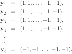
Hence, for a given judge the experiment results in one of 2p(J2) =ℓpossible response pattern

vectorsyi,i = 1,2, . . . , ℓ, a vector ofp J₂

the pre-defined order (1). In general the response pattern vector can be written as

y= (y121, y122, . . . , y12p;y131, y132, . . . , y13p;. . .;yJ−1,J,1, yJ−1,J,2, . . . , yJ−1,J,p),

withyijα∈ {1,−1}according to (4). The order in which the responses are observed could be the standard order of a 2p(J2) factorial main effects only design; this means that the

rightmost y varying the fastest and the leftmost y varying the slowest with all possible combinations being produced. A few response pattern vectors are then given by

y₁ = (1,1, . . . , 1, 1),

y₂ = (1,1, . . . , 1,−1),

y₃ = (1,1, . . . ,−1, 1),

y₄ = (1,1, . . . ,−1,−1), ..

.

yℓ = (−1,−1, . . . ,−1,−1).

In order to get a log-linear representation for the multivariate paired comparison experiment that can be extended to account for the mentioned dependencies we have to model the joint distribution of the the random variable

Y={Y121, Y122, . . . , Y12p;Y131, Y132, . . . , Y13p;. . .;YJ−1,J,1, YJ−1,J,2, . . . , YJ−1,J,p}.

Example: To illustrate the log-linear approach consider the special caseJ = 3 andp= 2. According to the multiplicative specification for multivariate binary data due to Cox (1972), we specify the joint probability distribution for the random variableYin the following way: by using Sinclair’s reparameterization (Sinclair(1982)) of the Bradley-Terry specification (3) for a single comparison

P{Yijα=yijα}=

1 p

πiα/πjα+ p

πjα/πiα

√_π

iα √_π

jα yijα

, yijα∈ {−1,1} (5)

we obtain the joint distribution analogously to Dittrich, Hatzinger and Katzenbeisser (2002):

P{Y121 = y121, Y122=y122;Y131 =y131, Y132=y132;Y231=y231, Y232=y232}=

= ∆

√_π

11 √_π

21

y121√_π 12 √_π

22

y122√_π 11 √_π

31

y131√_π 12 √_π

32

y132√_π 21 √_π

31

y231√_π 22 √_π

32 y232

×

exp{θ1,23|1y121y131}exp{θ1,23|2y122y132} ×

exp{θ2,13|1y121y231}exp{θ2,13|2y122y232} × (6) exp{θ3,12|1y131y231}exp{θ3,12|2y132y232} ×

exp{β12|12y121y122}exp{β13|12y131y132}exp{β23|12y231y232},

FIGURE 1 ABOUT HERE

Figure 1: Dependency structure

Furthermore, letNibe the random variable

Ni= number of times where response pattern vectoryi, i= 1,2, . . . , ℓ , occurs,

then theNi’s are multinomially distributed withN=P

iNi, and probabilities given in (6). Now let mi be the expectation of Ni, i.e. the expected number of times where response pattern vectory_ioccurs. Hence we base our estimation procedure upon simple multinomial sampling. Thus we obtain for the logarithm of the expectationmi of the random variables Nithe following linear representation

lnm = γ+λ11(y121+y131) +λ12(y122+y132) +

λ21(y231−y121) +λ22(y232−y122) +

λ31(−y131−y231) +λ32(−y132−y232) +

θ1,23|1y121y131+θ1,23|2y122y132+ (7) θ2,13|1y121y231+θ2,13|2y122y232+

θ3,12|1y131y231+θ3,12|2y132y232+

β12|12y121y122+β13|12y131y132+β23|12y231y232,

where γ = ln ∆ and λiα = 1₂lnπiα. For example, the log-linear representation for the expectation ofN1, the expected number of times, where the response pattern vectory₁= (1,1; 1,1; 1,1) occurs is given by

lnm1 = γ+ 2λ11+ 2λ12−2λ31−2λ32+

θ1,23|1+θ1,23|2+θ2,13|1+θ2,13|2+θ3,12|1+θ3,12|2+ β12|12+β13|12+β23|12.

Model (7) is a Generalised Linear Model and the parameters can easily be estimated by standard software using, e.g. by GLIM using Poisson error and a log-link. The design matrix for the case under considerations, is given by

X= (1,YA,W), (8)

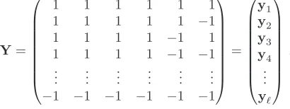
where 1 is a column vector consisting of 1. The (26_{×6)-matrix Y, the response pattern} matrix, is the design matrix for a 26_{main effects only design in standard order (in fact the} rows ofYare the response pattern vectorsyi and is given by

Y=         

1 1 1 1 1 1

1 1 1 1 1 −1

1 1 1 1 −1 1

1 1 1 1 −1 −1

..

. ... ... ... ... ... −1 −1 −1 −1 −1 −1

         =          y₁ y₂ y3 y₄ .. . yℓ          , and

where B is the (3×3) paired comparison design matrix (B¨ockenholt and Dillon (1997)). Each column of this matrix corresponds to one of the 3 objects, and each row to one of the

3 2

= 3 paired comparisons (in the order given in (1))

B= 



1 −1 0

1 0 −1

0 1 −1



;

I2denotes the (2×2) identity matrix, and the index refers to the number of attributes, i.e, p= 2. The matrixWis given byW= (W1,W2), where the columns ofW1represent the between object pairs dependencies, and the columns ofW2 represents the within attribute dependencies, according to our previous definition. Therefore, all columns of the matrixW

can be interpreted as representing two-way interactions between responses corresponding to columns ofYand can easily be constructed in the usual GLM way as two-way interactions by elementwise multiplication of suitable columns of the response pattern matrix Y. Let

y_ijα be the columns of the response pattern matrix, corresponding to the comparison of objectsiandj on attributeα, i.e. Y= (y₁₂₁,y₁₂₂;y₁₃₁,y₁₃₂;y₂₃₁,y₂₃₂), the matricesW1 andW2are given by

W1= (y121⊙y131,y122⊙y132,y121⊙y231,y122⊙y232,y131⊙y231,y132⊙y232),

and

W2= (y121⊙y122,y131⊙y132,y231⊙y232),

where⊙represents the elementwise (Hadamard) product of the corresponding columns. The design matrix for the simplest case as shown in the example can be generalized for more than three objects and more than two attributes in an obvious way. For the general case withJ objects andpattributes the design matrix is analogously to (8) given by

X= (1,YA,W)

where the matrixYis the (2p(J2)×p J

2

) design matrix for a 2p(J2) main effects only design

in standard order,A=B_⊗Ip, whereBis the ( J₂

×J) paired comparison design matrix given by B=     

1 −1 0 . . . 0 0 1 0 −1 . . . 0 0 ..

. ... ... . . . ... ... 0 0 0 . . . 1 −1

     ,

andIpis the corresponding identity matrix of orderp, i.e. the number of attributes. Care has only to be taken when specifying the matrix Wbecause not all possible interactions between columns ofYare meaningful according to the definition of the origin causing the dependencies as there are nonoverlapping sets of object indices, whenJ≥4. The log-linear model is overparameterized and one has to impose some restrictions on the parameters. In this paper we use the standard GLIM-restrictions, and aliase theλparameters accordingly.

2.2. Parameter interpretation

in the hypothesis θ1,23|α = θ1,24|α = · · · = θ1|α. Another, more restrictive

hypoth-esis, would be θ1|1 = θ1|2 = · · · = θ1|p = θ1|·. Furthermore, another hypothesis is

θ1,23|1 = θ1,23|2 = · · · = θ1,23|p. The most restrictive hypothesis would be that all

asso-ciation parameters are zero, in which case the independence model is achieved. It might also be of interest whether theβ-parameters can be restricted in some interesting way. An obvious advantage of this GLM-approach is that all mentioned hypotheses can easily be tested in the usual GLM way by comparing deviances of the associated nested models.

The interpretation of the parameters of model (7) is best seen by considering conditional distributions, because as Cox pointed out, conditional distributions from this class of models have a simple form, marginal probabilities do not. Consider for example the log-odds in favour ofY121 conditional on all otherYijα:

ln P{Y121= 1|Y

−

} P{Y121=−1|Y−}

= 2(λ11−λ21) + 2(θ1,23|1y131+θ2,13|1y231) + 2β12|12y122,

where Y− denotes the random vectorY without the elementY121. Therefore, for given attributeα= 1, the log-odds in favour of objectO1are not only determined by the param-eters of the involved objects, as in the basic BT-model, but additionally (i) allθ’s have to be taken into account which represents interactions between those pairs of paired comparisons which involve the pair (O1, O2), i.e. the pairs ((O1, O2),(O1, O3)) and ((O1, O2),(O2, O3)), and (ii) there is perhaps also an effect of the within attribute dependency. Therefore, for two evenly matched objects, and assuming no within attribute dependency, i.e. β12|12= 0, there is an advantage in preferring objectO1 over objectO2 regarding attribute α= 1 if θ1,23|1y131+θ2,13|1y231>0, which for example is given whenθ1,23|1and θ2,13|1are positive and y131 = y231 = 1. Note that this advantage is caused solely by the assumed between object pairs dependency.

Theθ-parameters are proportional to log-odds ratios describing the association between two Y’s in the conditional distribution of two paired comparisons, i.e. two Y’s, given the others. For example, the parameterθ1,23|1 is proportional to the log-odds ratio in the conditional distribution of{Y121, Y131}givenY−, whereY−now denotes the random vector

Ywithout the elements{Y121, Y131}:

lnP{Y121= 1, Y131= 1|Y

−

}P{Y121=−1, Y131=−1|Y−} P{Y121= 1, Y131=−1|Y−}P{Y121=−1, Y131= 1|Y−}

= 4θ1,23|1.

A positive association parameterθ1,23|1 indicates that the judges will rather be consistent (positive or negative) within their decisions between objectsO1andO2for a given attribute. Following B¨ockenholt and Dillon (1997) theθparameters can be interpreted as an indicator of a stimulus identity effect that reflects the degree of similarity or consistency in the two assessments of the common object with regard to the attribute. In general, however, the interpretation of the sign of the association parametersθis not so straight forward, because it depends on the object indices involved in the pairs of paired comparisons. If the common indexiis the smallest or the largest of the involved indicesi, j, kthan a positive parameter suggests consistency of the decisions, but in all other cases a negative parameter indicates consistency. This is caused by the ordering of the two-dimensional tables representing the two-dimensional conditional distributions of the random variables Yij|α and Yik|α, as will

be shown in the following example.

Y’s:

ln P{Y121= 1, Y122= 1|Y

−

}P{Y121=−1, Y122=−1|Y−} P{Y121= 1, Y122=−1|Y−}P{Y1211=−1, Y122= 1|Y−}

= 4β12|12.

A positive (negative) parameter β12|12indicates therefore a positive (negative) association between both attributes within the comparison of objects 1 and 2, given all other decisions.

3. An Application

In this section we will illustrate our approach by means of an example. A paired comparison experiment was carried out at the Vienna University of Economics during the summer term 2001, after the election in the year 1999. 266 mainly first-year students were asked to state a preference about the leaders of the four political parties represented in the Austrian Parliament. In this experiment two attributes, namelycompetence in social issues, s,and

competence in economic issues, e,were taken into account. The leaders of the four political parties are denoted by the abbreviations S, the head of the social democrats, F, the leader of the so-called freedom party , C, the leader of the conservatives, and G the head of the green (ecologic) party (sorted by the number of votes reached in the election 1999). Two questions for each pairwise comparison were asked, namely which of two party leaders has more competence in social issues and more competence in economic issues, respectively.

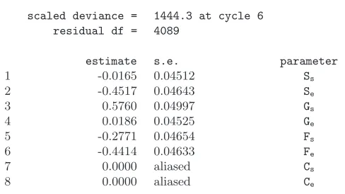
As a first step the independence model for four items (=party leaders) was fitted by GLIM and the results are given in Table 3 in the appendix. From the estimates of the initialλ parameters the worth parameters ˆπ for the four party leaders with respect to the two attributes can be calculated by

ˆ

πiα= exp{2ˆλ iα} P

ℓexp{2ˆλℓα} and are shown in the following table:

ˆ πs πˆe G 0.55 0.37 C 0.18 0.35 S 0.17 0.14 F 0.10 0.14

From the independence model one would conclude that G, the leader of the Green party, is thought to have the most competence in social and economic issues. However, the distance to C in the economic attribute is not significant; an approximate 0.95%-confidence interval for the initial parameterλGeis given by [−0.072,0.109]. S and F are quite similar, although S is seen to have a higher social competence, the corresponding approximate 0.95%-confidence interval forλSs is given by [−0.106,0.074]. One has to be careful in interpreting the overall fit of the independence model because there are numerous random zeros in the underlying contingency table, which inflates the residual degrees of freedom. Therefore we consider deviance changes of hierarchical models only.

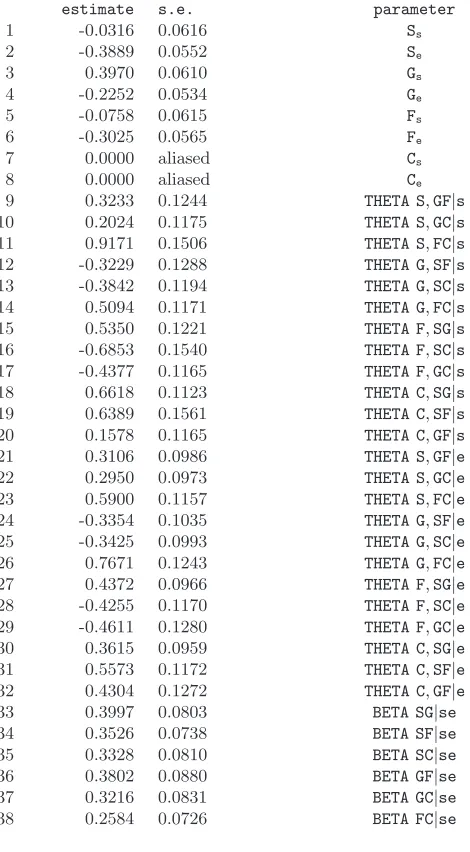
a tremendous improvement of the fit, with a change of deviance 813.3 on 30 degrees of freedom. This suggests that the independence model is not appropriate for this data set. It is interesting that the worth parameters for the party leaders based on this dependence model change:

ˆ πs πˆe G 0.44 0.24 C 0.20 0.38 S 0.19 0.17 F 0.17 0.21

The changes in the model parameters are displayed in Figure 2, where the arrows represent the direction of the changes, with starting points given by the worth parameters calculated on the basis of the independence model.

FIGURE 2 ABOUT HERE

Figure 2: Ascribed competence in social and economic issues

The effect of the incorporation of the dependencies leads to, at least in this example, more similarity between the party leader, which can be seen in Figure 2. The ascribed competence of G, the head of the green party, changes most. Compared to the initial model he is seen to be less competent in both attributes, but still he is ascribed the highest competence in social issues of all party leaders; an approximate 0.95% confidence interval for the corresponding initial social competence parameter is given by [0.275; 0.519]. C gains in both attributes and overtakes G in the ascribed competence in economic issues.

Concerning the interaction parametersθ they have positive as well as negative signs. Nevertheless, all those interaction parameters indicate that there is a tendency towards consistent decisions. Consider for example the parametersθS,GF|s andθF,SC|s. To make it

easier to read we will denote the choices e.g. {YSF s= 1}, if the first leader (S) is chosen, by SF >sS and and the choice{YSF s=−1}, if the second leader (F) is chosen, bySF >s F. The (estimated) parameter ˆθS,GF|simplies that the (estimated) choice probabilities can be written as:

P{SG >sS, SF >s S|Y−}P{SG >sG, SF >sF|Y−}=

exp{4·0.3233} P{SG >sS, SF >sF|Y−}P{SG >sG, SF >sS|Y−}.

SF >sS both mean that S, the first party leader in the comparisons is seen to have more competence in social issues (s) when compared to F and G whileSF >s F and SG >s G mean that in both cases S is seen to have less competence in social issues when compared to F and G. Whereas the responses in the other side are inconsistent decisions about S, because S is seen to have more competence in social issues than F (SF >s S) but less competence in social issues than G (SG >sG). This illustrates that in this case the chance for a consistent decision ({SF >s S, SG >s S}{SF >s F, SG >s G}) of the students for either always choosing S to be the party leader with more competence in social issues or never choosing S when compared to the party leaders F or G is exp{1.2932}= 3.64 times higher than the probability for choosing S just once when compared to the party leader F or G. In other words one is more likely either to prefer the social democrat to both the conservative and freedom party leader, or to prefer the freedom and conservative party leader to the social democrat.

On the other hand forθF,SC|s we get

P{SF >s S , F C >s F|Y−}P{SF >sF, F C >sC|Y−}=

exp{−4· 0.6853}P{SF >sS, F C >sC|Y−}P{SF >sF, F C >sF|Y−}.

In this case consistency about the leader F is indicated by{SF >s S, F C >s C}{SF >s F, F C >s F}which is now on the right hand side of the formula above, and therefore the chance for consistency is 1

exp{−4·0.6853}≈16 times higher than the chance for inconsistency.

In order to obtain a more parsimonious model, we tried to simplify theθ’s, according to the suggestions made at the end of Section 2. However, in general this is not possible in this example. Consider for example the hypothesisθS,GF|s =θS,GC|s =θS,F C|s =θS|s.

This hypothesis has to be rejected, change in deviance is 18.7 on 2 df. This is the reason why we did not simplify the model further with respect to theθparameters.

It is also remarkable that allβ-parameters are positive and approximately of the same size. Therefore the model can further be simplified by substituting six parameters by only oneβ, with an estimated value of 0.3385 (s.e.=0.0297), change in deviance is 2.03 on 5 df. This can be interpreted as a positive association between the competence in social- and economic issues.

Summarizing the results of this experiment one could conclude that it is important to consider interaction parameters representing dependencies between the decisions of the judges on the one hand and attributes on the other hand, otherwise one might get biased estimates for the worth parameters.

4. Acknowledgements

5. References

Agresti, A., 1990. Categorical Data Analysis. J.Wiley, New York.

Agresti, A., 1992. Analysis of ordinal paired comparison data. Applied Statistics, 41, 287-297.

Bahadur, R. R., 1961. A representation of the joint distribution of responses ton dichoto-mous items. In: Solomon, H. (Eds.), Studies in Item Analysis and Prediction. Stanford University Press, Stanford, pp. 158-176,

B¨ockenholt, U., 1988. A Logistic Representation of Multivariate Paired-Comparison Mod-els. Journal of Mathematical Psychology, 32, 44-63.

B¨ockenholt, U. and W. Dillon, 1997. Modelling within-subject dependencies in ordinal paired comparison data. Psychometrika, 62, 411-434.

Bradley, R. A. and M. E. Terry, 1952. Rank analysis of incomplete block designs I. The method of paired comparisons. Biometrika, 39, 324-345.

Cox, D., 1972. The analysis of multivariate binary data. Applied Statistics, 21, 113-120. David, H. A., 1988. The Method of Paired Comparisons, 2nd ed. Griffin, London.

Davidson, R. R., 1970. Extending the Bradley-Terry model to accommodate ties in paired comparison experiments. Journal of the American Statistical Association, 65, 317-328. Davidson, R. R. and R. A. Bradley, 1969. Multivariate paired comparisons: The extensions of a univariate model and associated estimation and test procedures. Biometrika, 56, 81-95. Davidson, R. R. and R. J. Beaver, 1977. On extending the Bradley-Terry model to incor-porate within-pair order effects. Biometrics, 33, 693-702.

Dittrich R., R. Hatzinger and W. Katzenbeisser, 1998. Modelling the effect of subject-specific covariates in paired comparison studies with an application to university ranking. Applied Statistics, 47, 511-525.

Dittrich, R., R. Hatzinger, and W. Katzenbeisser, 2002. Modelling dependencies in paired comparison experiments. A log-linear approach. Computational Statistics & Data Analysis, 40, 39-57.

Fienberg, S. E., 1979. Log linear representation for paired comparison models with ties and within-pair order effects. Biometrics, 35, 479-481.

Francis, B. et.al (Eds.) 1993. The GLIM System. Release 4 Manual. Clarendon Press, Oxford.

Francis B. R. Dittrich , R. Hatzinger and R. Penn, 2002. Analysing partial ranks by using smoothed paired comparison methods: an investigation of value orientation in Europe. Applied Statistics, 51, 319-336.

Grizzle, J. E., Starmer, C. F. and G. G. Koch, 1969. Analysis of categorical data by linear models. Biometrics, 25, 489-504.

Imrey, P. B., W. D. Johnson, and G. G. Koch, 1976. An incomplete contingency table ap-proach to paired-comparison experiments. Journal of the American Statistical Association, 71, 614-623.

Kousgaard, N., 1976. Models for paired comparisons with ties. Scandinavian Journal of Statistics, 3, 1-11.

Kousgaard, N., 1984. Analysis of a sound field experiment by a model of paired comparisons with explanatory variables. Scandinavian Journal of Statistics, 11, 243-255.

Matthews, J. N. S. and K. P. Morris, 1995. An application of Bradley-Terry-type models to the measurement of pain. Applied Statistics,44, 243-255.

Sinclair, C. D., 1982. GLIM for preference. In: Gilchrist, R. (Eds.): GLIM 82. Proceedings of the International Conference on Generalised Linear Models. Springer Lecture Notes in Statistics, 14. pp. 164-178.

Table 1. Estimates of the λparameters of the independence multivariate model

scaled deviance = 1444.3 at cycle 6 residual df = 4089

estimate s.e. parameter

1 -0.0165 0.04512 Ss

2 -0.4517 0.04643 Se

3 0.5760 0.04997 Gs

4 0.0186 0.04525 Ge

5 -0.2771 0.04654 Fs

6 -0.4414 0.04633 Fe

7 0.0000 aliased Cs

Table 2. Parameter estimates for the multivariate dependence model

scaled deviance = 630.98 (change = -813.3) at cycle 8 residual df = 4059 (change = -30 )

estimate s.e. parameter

1 -0.0316 0.0616 Ss

2 -0.3889 0.0552 Se

3 0.3970 0.0610 Gs

4 -0.2252 0.0534 Ge

5 -0.0758 0.0615 Fs

6 -0.3025 0.0565 Fe

7 0.0000 aliased Cs

8 0.0000 aliased Ce

9 0.3233 0.1244 THETA S,GF|s

10 0.2024 0.1175 THETA S,GC|s

11 0.9171 0.1506 THETA S,FC|s

12 -0.3229 0.1288 THETA G,SF|s 13 -0.3842 0.1194 THETA G,SC|s

14 0.5094 0.1171 THETA G,FC|s

15 0.5350 0.1221 THETA F,SG|s

16 -0.6853 0.1540 THETA F,SC|s 17 -0.4377 0.1165 THETA F,GC|s

18 0.6618 0.1123 THETA C,SG|s

19 0.6389 0.1561 THETA C,SF|s

20 0.1578 0.1165 THETA C,GF|s

21 0.3106 0.0986 THETA S,GF|e

22 0.2950 0.0973 THETA S,GC|e

23 0.5900 0.1157 THETA S,FC|e

24 -0.3354 0.1035 THETA G,SF|e 25 -0.3425 0.0993 THETA G,SC|e

26 0.7671 0.1243 THETA G,FC|e

27 0.4372 0.0966 THETA F,SG|e

28 -0.4255 0.1170 THETA F,SC|e 29 -0.4611 0.1280 THETA F,GC|e

30 0.3615 0.0959 THETA C,SG|e

31 0.5573 0.1172 THETA C,SF|e

32 0.4304 0.1272 THETA C,GF|e

33 0.3997 0.0803 BETA SG|se

34 0.3526 0.0738 BETA SF|se

35 0.3328 0.0810 BETA SC|se

36 0.3802 0.0880 BETA GF|se

37 0.3216 0.0831 BETA GC|se