R E S E A R C H
Open Access
Asymptotic expansions of the error for
hyper-singular integrals with an interval
variable
Chong Chen
*, Jin Huang and Yanying Ma
*Correspondence: [email protected]
School of Mathematical Sciences, University of Electronic Science and Technology of China, Qingshuihe Campus, Chengdu, 611731, China
Abstract
In this paper, we present high accuracy quadrature formulas for hyper-singular integralsabg(x)qα(x,t)dx, whereq(x,t) =|x–t|(orx–t),t∈(a,b), and
α
≤–1 (orα
< –1). Ifg(x) is 2m+ 1 times differentiable on [a,b], the asymptotic expansions of the error show that the convergence order isO(h2μ+1+α) withq(x,t) =|x–t|(orx–t) forα
≤–1 (orα
< –1 andα
being non-integer), and the error power isO(hη) withq(x,t) =x–tfor
α
being integers less than –1, whereη
= min(2μ
, 2μ
+ 2 +α
) andμ
= 1,. . .,m. Since the derivatives of the density functiong(x) in the quadrature formulas can be eliminated by means of the extrapolation method, the formulas can easily be applied to solving corresponding hyper-singular boundary integral equations. The reliability and efficiency of the proposed formulas in this paper are demonstrated by some numerical examples.MSC: 45E99; 65D30; 65D32; 41A55
Keywords: hyper-singular integral; Euler-Maclaurin expansions; quadrature formulas; Hadamard finite part
1 Introduction
We consider the following hyper-singular integral with an interval variablet∈(a,b):
I(g)(t) = b
a
g(x)qα(x,t)dx, (.)
whereq(x,t) =|x–t|(orx–t), andα≤– (orα< –) is a real number. Equation (.) denotes the Hadamard finite part [, ] of the hyper-singular integral. Hyper-singular in-tegrals have been extensively used to elasticity problems [, ], for example, the calcula-tion of stresses. Hyper-singular integral operators also attracted attencalcula-tion such as in [] on modulation spaces. Especially, in the boundary element method, the hyper-singular integrals have attracted considerable attention such as in [, , ]. The authors of [] ap-ply boundary integral equations for the solution of the electrostatic field problem floating potentials in industrial applications.
So far, many numerical methods have been proposed to evaluate the hyper-singular in-tegral (.) forα= –. According to the quadrature rules based on interpolation trigono-metric polynomials, Kim and Choi gave two quadrature formulas for evaluating (.) with
α= – in [], in which the cosine transform of variables and trigonometric polynomial interpolation at the practical abscissa were used, where a three-term recurrence relation was used to evaluate the quadrature weights. In [], Huanget al.got the Euler-Maclaurin expansions of (.) with –≤α< – by a modified trapezoidal formula. In [], Kabiret al.
used the piecewise quadratic polynomial technique to solve integral equations with loga-rithmic, Cauchy, and hyper-singular integrals. Hui and Shia presented a Gaussian quadra-ture formula for (.) withq(x,t) =|x–t|forα= –, where the classical orthogonal poly-nomials such as the Legendre and Chebyshev polypoly-nomials were used in []. In [], the hyper-singular integral equations were applied to solving the flat crack problem. On the basis of Euler-Maclaurin expansions in [], Sidi and Israeli got the quadrature formulas and the error asymptotic expansions of the integral (.) with q(x,t) =x–tforα= –. In , Monegato and Lyness obtained the Euler-Maclaurin expansions of (.) by the Mellin transform, ast= andα< –.
The quadrature formulas in [] are not valid for solving hyper-singular integral equa-tions and are only valid at the endpoint of the integrand interval. In this paper, by gen-eralizing the results of Monegato and Lyness in , we extend the formulas to any in-terior point of the integrand interval, and we present high accuracy quadrature formulas for hyper-singular integralsabg(x)qα(x,t)dx, whereq(x,t) =|x–t|(orx–t),t∈(a,b), and
α≤– (orα< –). Ifg(x) is m+ times differentiable on [a,b], the asymptotic expansions of the error show that: (i) whenα≤– (orαis a non-integer less than –), the convergence order isO(hμ++α) withq(x,t) =|x–t|(orx–t), whereμ= , . . . ,m; (ii) whenαis an integer
less than –, the error power isO(hη) withq(x,t) =x–t, whereη=min(μ, μ+ +α) and
μ= , . . . ,m. Since the derivatives of the density functiong(x) in the quadrature formulas can be removed by means of the extrapolation method, the formulas can easily be applied to solving the corresponding hyper-singular boundary integral equations. Quadrature for-mulas can also be used to solve singular integral equations in its corresponding forms. The hybrid Gauss-trapezoidal quadrature rule [] is one of many quadrature formulas. There are also several methods to solve hyper-singular boundary integral equations beside quadrature rules, such as potential theory [], the Green function approach [], and so on. As far as this paper is concerned, we only deal with hyper-singular integrals. Moreover, numerical results display the significance of these formulas proposed, finally.
This paper is organized as follows: in Section , we introduce the Euler-Maclaurin ex-pansions for hyper-singular integrals of (.) at the end points of the integrand interval; in Section , we present high accuracy quadrature formulas for hyper-singular integrals (.) with an interval variable, and also we get their Euler-Maclaurin expansions; in Section , some numerical examples are tested. A few conclusions are drawn in Section .
2 Euler-Maclaurin expansions for integrals of (2.1) at end points
In this section, we will recall some notations and extend the results of []. In [], Monegato and Lyness presented the expansion of integrals whose integrand function is singular or hyper-singular at the end points of the integrand interval [, ]. We extend the results to any interior point of the integrand interval [a,b].
We discuss the following integrals:
b
a
whereg(x)∈Cm[a,b] andω=min(α,γ)≤–. Note that
f.p. b
a
f(x,t)dx=f.p. b
a
(x–a)α(b–x)γg(x)dx, (.)
wheref.p. denotes theHadamard finite part[] of the integral. Whenω= –, (.) is a singular integral. Whenω< –, (.) is a hyper-singular integral. By using the results of [], we derive the Euler-Maclaurin expansion of (.).
Lemma . Assume that g(x)is m times differentiable on[a,b]and f(x) = (x–a)α(b–
x)γg(x),withω=min(α,γ)≤–.n is the number of nodes in the rules,and h=b–a n .Then
the following expansions hold.
(i)Ifαandγ are non-integer,we have
h
n–
k=
fa+h(β+k)–
m
k=
hk++α
k! ζ(–k–α,β)g (k) (a)
–
m
k=
(–)khk++γ
k! ζ(–k–γ, –β)g (k) (b)
=f.p. b
a
f(x)dx+ πi
c+i∞
c–i∞
h–pF˜(p) +F˜(p)
ζ(p,β)dp. (.)
(ii)Ifα= –l– ,l= , , . . . ,andγ is non-integer,the formula is
h
n–
k=
fa+h(β+k)–
m
k=,k=l
hk++α
k! ζ(–k–α,β)g (k) (a)
–
m
k=
(–)khk++γ
k! ζ(–k–γ, –β)g (k) (b)
+g (l) (a)
l! ψ(β) –
g(l)(a)
l! ln
h
=f.p. b
a
f(x)dx+ πi
c+i∞
c–i∞
h–pF˜(p) +F˜(p)
ζ(p,β)dp. (.)
(iii)Whenγ = –l– ,l= , , . . . ,andαis a non-integer,the expansion can be written
h
n–
k=
fa+h(β+k)–
m
k=
hk++α
k! ζ(–k–α,β)g (k) (a)
–
m
k=,k=l
(–)khk++γ
k! ζ(–k–γ, –β)g (k) (b)
+ (–)lg (l) (b)
l! ψ(β) – (–)
lg
(l) (b)
l! ln
h
=f.p. b
a
f(x)dx+ πi
c+i∞
c–i∞
h–pF˜(p) +F˜(p)
(iv)Whenα= –l– ,γ= –s– ,l and s are integers,we have the form
h
n–
k=
fa+h(β+k)–
m
k=,k=l
hk++α
k! ζ(–k–α,β)g (k) (a)
–
m
k=,k=s
(–)khk++γ
k! ζ(–k–γ, –β)g (k) (b) +
g(l)(a)
l! ψ(β)
–g (l) (a)
l! ln
h+ (–)
sg
(s) (b)
s! ψ( –β) – (–)
sg
(s) (b)
s! ln
h
=f.p. b
a
f(x)dx+ πi
c+i∞
c–i∞
h–pF˜(p) +F˜(p)ζ(p,β)dp, (.)
where <β< ,ζ(p,β) =∞k=(k+β)–p(Re(p) > )is the Riemann zeta function,F˜ i(p) =
∞
fi(x)xp–dx (i= , )is the Mellin transform, and the other functions are defined by
ψ(β) =(β)/(β),g(x) = (b–x)γg(x),g(x) = (x–a)αg(x),c∈[–m–ω– , –m–ω– ],
f(x) =f(x)v(x; /, /),f(x) =f(x)( –v(x; /, /)),and f(x) =f( –x).We also define v(x,k,k) (k<k)such that v(x,k,k)belongs to C∞(–∞,∞)and
v(x,k,k) = ⎧ ⎨ ⎩
for x≤k, for x≥k.
Proof Considering the hyper-singular integrals (.) and takingy= – (b–x)/(b–a), we obtain
b
a
(x–a)α(b–x)γg(x)dx=
yα( –y)γg˜(y)dy=
˜
f(y)dy,
whereg˜(y) = (b–a)+α+γg(a+ (b–a)y) andf˜(y) =yα( –y)γg˜(y) =f(a+ (b–a)y). According
to the conclusions of [], we obtain the results of Lemma ..
Obviously, the quadrature formulas can be derived by Lemma .. To get the conver-gence order of the quadrature rules, we estimate the value of
πi
c+i∞
c–i∞ h
–pF˜(p) +F˜(p)ζ(p,β)dp
as Corollary ..
Corollary . Under the assumptions of Lemma.,
Rc,p= πi
c+i∞
c–i∞
h–pF˜(p) +F˜(p)ζ(p,β)dp
=oh–c=ohRe(α)+m+, n→ ∞, (.)
Proof Letp=c+is, thus
Rc,p= πi
∞
–∞h
–c–isF˜
c+is+F˜
c+isζc+is,βi ds
=h –c
π
∞
–∞
h–isF˜
c+is+F˜
c+isζc+is,βds.
Based on the definition ofF˜i(p),i= , , we have
∞
–∞
h–isF˜
c+is+F˜
c+isζc+is,βds<c,
thenR(c,p) =o(h–c) asn→ ∞, wherecis a constant number. 3 Quadrature formulas of hyper-singular integrals and their Euler-Maclaurin
expansions
In this section, we study the following integrals:
I(G) =f.p. b
a
G(x,t)dx=f.p. b
a
qα(x,t)g(x)dx, (.)
I(G) =f.p. b
a
G(x,t)dx=f.p. b
a
|x–t|αln|x–t|pg(x)dx, α< –, (.)
whereq(x,t) =|x–t|(orx–t) forα≤– (orα< –), andpis a nonnegative integer,g(x) is a smooth function on [a,b].G(x,t) andG(x,t) are hyper-singular functions about interval variabletasα< –.
We divide the interval [a,b] intonequal parts, that is,h= (b–a)/n. Letxj=a+jh(j=
, , . . . ,n) and the singular pointtsatisfiest∈ {xj: ≤j≤n– }, and we also takeβ= /.
In terms of Lemma . and the classic Euler-Maclaurin expansions on modified trapezoidal formulas, we derive the following formulas of the integral (.) withq(x,t) =|x–t|.
Theorem . Suppose g(x)ism+ times differentiable on[a,b],G(x,t) =g(x)|x–t|αwith
α≤–,and t∈ {xj: ≤j≤n– }.Then the modified rule is
Q(h) =
n–
j=
hG
a+
j+
h
– h+αζ
–α,
g(t), (.)
at the same time the following assertions hold.
(i) Ifαis a non-integer,the error expansion can be written
En(h) =I(G) –Q(h)
=
m+
k=
hkB
k()
(k)!
G(k–)(a) –G(k–)(b)
–
m
k=
hk++α
(k)! ζ
–k–α,
g(k)(t) +Ohm+α+, (.)
(ii) Whenα= –l– withl∈N,the error expansion is given by
En(h) = m+
k=
hk
(k)!Bk
G(k–)(a) –G(k–)(b)
–
m
k=,k=l
h(k–l) (k)!ζ
(l–k) + ,
g(k)(t)
+ g (l)(t) (l)! ψ
– g
(l)(t) (l)! ln
h+O
hm++α. (.)
(iii) Asα= –lwithl∈N+,we obtain the error expansion of the form
En(h) = m+
k=
hk
(k)!Bk
G(k–)(a) –G(k–)(b)
–
min(m,l–)
k=
h(k–l)+ (k)! ζ
(l–k),
g(k)(t) +Ohm++α, (.)
whereEn(h) =I(G) –Q(h)andψ(/) = –. – ln.
Proof Taket=xi, thentis an interior point of division of the interval (a,b). The integral
of (.) can be decomposed into two parts
f.p. b
a
G(x,t)dx=f.p. b
a
g(x)|x–t|αdx
=f.p. t
a
g(x)(t–x)αdx+f.p. b
t
g(x)(x–t)αdx. (.)
We consider the first item of the theorem at first. By equations (.) of Lemma . and (.) of Corollary ., we have
i– j= hG a+
j+
h
=f.p.
t
a
G(x,t)dx
+
m
k=
hk
(k– )!ζ
–k+ ,
G(k–)(a)
+ m+
k=
(–)khk++α
k! ζ
–k–α,
g(k)(t) +Ohm++α (.)
and
n–
j=i
hG
a+
j+
h
=f.p.
b
t
G(x,t)dx
–
m+
k=
hk
(k– )!ζ
–k+ ,
G(k–)(b)
+ m+
k=
hk++α
k! ζ
–k–α,
Combining (.) with (.), we obtain n– j= hG a+
j+
h
=f.p.
b
a
G(x,t)dx
+
m+
k=
hk
(k– )!ζ
–k+ ,
G(k–)(a) –G(k–)(b)
+
m
k= h
k++α
(k)! ζ
–k–α,
g(k)(t) +Ohm++α. (.)
Since
ζ
–k,
= , ζ
–k– ,
= –Bk+( )
k+ , k= , , , . . . , we have the forms of (.) and (.).
Next, we will derive the conclusions of (ii) and (iii). Using the rules of (.), (.), and (.), we get the corresponding formulas:
i– j= hG a+
j+
h
=f.p.
t
a
G(x,t)dx–
m+
k=
hk
(k)!Bk
G(k–)(a)
– (–)–α–g (–α–)(t) (–α– )!ψ
+ (–)–α–g (–α–)(t) (–α– )!ln
h
+ m+
k=,k=–α–
(–)khk++α
k! ζ
–k–α,
g(k)(t)
+Ohm++α (.)
and
n–
j=i
hG
a+
j+
h
=f.p.
b
t
G(x,t)dx+
m+
k=
hk
(k)!Bk
G(k–)(b)
–g (–α–)(t) (–α– )!ψ
+g (–α–)(t) (–α– )!ln
h
+ m+
k=,k=–α–
hk++α
k! ζ
–k–α,
g(k)(t)
+Ohm++α. (.)
Combining (.) with (.), we have
n– j= hG a+
j+
h
=f.p.
b
a
G(x,t)dx
+
m+
k=
hk
(k)!Bk
–(–)–α–+ g (–α–)(t) (–α– )!ψ
–g
(–α–)(t) (–α– )!ln
h
+ m+
k=,k=–α–
(–)k+ h
k+α+
k! ζ
–k–α,
g(k)(t)
+Ohm++α. (.)
It is easy to obtain the formula of the form
n– j= hG a+
j+
h
=f.p.
b
a
G(x,t)dx– g (l)(t) (l)! ψ
+ g (l)(t) (l)! ln
h+
m+
k=
hk
(k)!Bk
G(k–)(b) –G(k–)(a)
+
m
k=,k=l
h(k–l)
(k)!ζ
(l–k) + ,
g(k)(t) (.)
from (.) forα= –l– . Hence, equations (.) and (.) hold. Asα= –l(l≥), we have
n– j= hG a+
j+
h
=f.p.
b
a
G(x,t)dx
+
m+
k=
hk
(k)!Bk
G(k–)(b) –G(k–)(a)
+
min(m,l–)
k=
h(k–l)+
(k)! ζ
(l–k),
g(k)(t)
+Ohm++α (.)
from the rules of (.).
This completes the proof of theorem.
Clearly, the convergence order of the quadrature form of (.) is O(hμ++α) (μ=
, , . . . ,m).
Corollary . Under the assumption of Theorem.and lettingα= –,the quadrature rule is given by
Q(h) =
n– j= hG a+
j+
h
+ g(t)ψ
– g(t)ln
h, (.)
and the form of the asymptotic error expansion is
En(h) = m
k=
hk
(k)!Bk
G(k–)(a) –G(k–)(b)
–
m
k=
hk
(k)!ζ
– k,
Proof Letl= of (.) and (.), then the results hold. We have discussed the case of the kernel functionq(x,t) =|x–t| above, while some modelings of the phenomena naturally require numerical schemes of the hyper-singular integral (.) withq(x,t) =x–t. In Theorem ., we will lay out the quadrature formulas of (.) withq(x,t) =x–tand demonstrate them.
Theorem . Let g(x)be Cm+ function on[a,b]and G(x,t) =g(x)(x–t)αforα< –.At
the same time,we take t=xi, ≤i≤n– ,then the following assertions hold.
(i) Whenα= –l– forl∈N+,the expansion is
Q(h) =
n–
j=
hG
a+
j+
h
=f.p. b
a
G(x,t)dx+
m+
k=
hk
(k)!Bk
G(k–)(b) –G(k–)(a)
+
min(m,l–)
k=
h(k–l)+ (k+ )!ζ
(l–k),
g(k+)(t) +Ohm++α. (.)
(ii) Whenα= –l– withl= ,the form of the rule can be written n–
j=
hG
a+
j+
h
=
m+
k=
hk
(k)!Bk
G(k–)(b) –G(k–)(a)
+f.p. b
a
G(x,t)dx+Ohm++α. (.)
(iii) Ifαis a negative even(or non-integer),the results are the same as the formulas of Theorem.(iii) (or(i)).
Proof Settingt=xi, we divide the integral into two parts, as in the following forms:
f.p. b
a
G(x,t)dx=f.p. b
a
g(x)(x–t)αdx
=f.p. t
a
(–)αg(x)(t–x)αdx+f.p.
b
t
g(x)(x–t)αdx.
The proof of the theorem is similar to Theorem .. The only one difference of the proof is that (–)αg(x) in the above formulas can be regarded asg(x). Therefore, by using (.),
(.) of Lemma ., and (.) of Corollary ., respectively, we obtain
i–
j=
hG
a+
j+
h
=f.p. t
a
G(x,t)dx–
m+
k=
hk
(k)!Bk
G(k–)(a)
– (–)–α–
((–)αg(t))(–α–) (–α– )! ψ
–((–)
αg(t))(–α–) (–α– )! ln
h
+ m+
k=,k=–α–
(–)khk++α
k! ζ
–k–α,
(–)αg(t)(k)
+Ohm++α (.)
and
n–
j=i
hG
a+
j+
h
=f.p.
b
t
G(x,t)dx+
m+
k=
hk
(k)!Bk
G(k–)(b)
–g (–α–)(t) (–α– )!ψ
+g (–α–)(t) (–α– )!ln
h
+ m+
k=,k=–α–
hk++α
k! ζ
–k–α,
g(k)(t)
+Ohm++α. (.)
Adding the rules of (.) and (.), we have the following form:
n–
j=
hG
a+
j+
h
=f.p.
b
a
G(x,t)dx
+
m+
k=
hk
(k)!Bk
G(k–)(b) –G(k–)(a)
–(–)–α–(–)α+ g (–α–)(t) (–α– )!ψ
–g
(–α–)(t) (–α– )!ln
h
+ m+
k=,k=–α–
(–)k+α+ h
k+α+
k! ζ
–k–α,
g(k)(t)
+Ohm++α. (.)
We complete the proof of Theorem . from (.).
The quadrature formulas and error expansions of (.) have been given in the front part of this section. While we study some boundary integral equations arising in many prob-lems, we notice that these are not only required for calculating the integrals of (.), but we also need to discuss the integrals with logarithmic functions just like (.) to solve the equations. From equations (.), (.), and (.), one can obtain the Euler-Maclaurin ex-pansions for hyper-singular integrals with logarithmic functions. We deal with them in another paper.
Remark (i) We note the terms
min(m,l–)
k=
h(k–l)+ (k+ )!ζ
(l–k),
g(k+)(t)
extrapolation method to take the terms away. LettingQ(h) =Ql,l=––α,l∈N+, the
mod-ified quadrature rule is
Q(h) =Q(h), Qi(h) =
(l–k)–Qi–(h) –Qi–(h)
(l–k)–– , (.)
wherek= , , . . . ,l– ,i= , . . . ,l, and the order of error ofQl(h) isO(h).
(ii) Considering equations (.), (.), (.), and (.), we can obtain better numerical results by the Richardson extrapolation or the Romberg extrapolation method just like the above item (i).
Now, taking Example . for example withl= , we will obtain the quadrature formula and its error expansion. The quadrature rule of (.) isQ(h) =jn=–hG(a+ (j+ /)h). Then thekth extrapolation is given by
⎧ ⎨ ⎩
Q()(h) = Q(h) –Q(h),
Q(k)(h) = [kQ(k–)(h
) –Q (k–)
(h)]/(k– ), ≤k≤m+ , (.)
and the corresponding asymptotic expansion of error is
E(nk)(h) =
m+
μ=k+
c(μk)hμ+Ohm++α, (.)
whereE(nk)(h) =I(g) –Q
(k) (h),c()
μ =
Bμ()(––μ)[G(μ–)(a)–G(μ–)(b)]
(μ)! (μ= , . . . ,m+ ), and
c(k)
μ =
k–μ–
k– c(μk–). Clearly,Q
(k)
(h) has a high convergence order ofO(h(k+)), wherek= , . . . ,m+ .
As is seen from (.), (.), (.), (.), (.), and (.), their error expansions contain the term [G(k–)(b) –G(k–)(a)]. IfG(x) is a periodic function, those related terms will vanish. Then the quadrature formulas with higher orders of accuracy can be achieved by a Romberg extrapolation. Furthermore, ifG(x,t) is not a periodic function, we can obtain better numerical results by using a Richardson extrapolation or a Romberg extrapolation method in a different way just like in our remark.
4 Numerical experiments
In this section, we will display several numerical experiments which are associated with the implementation of the quadrature formulas proposed in this paper. The numerical results for non-periodic hyper-singular integrals are given. Leth=b–na be the step length used in the quadrature, wherenis the number of nodes.hk–ex(k= , , , ) are the
absolute errors of thekth extrapolation, andr(kn)= hk–ex (h)k–ex.
Example . Calculate the hyper-singular integral
I(g)(t) =
g(x)
(x–t)dx, g(x) = (x– )
, t∈(, ), (.)
where the exact solution is
Table 1 The numerical results fort= 0.25
ex\e\n 23 24 25 26 27 28
h0–ex 2.331e–2 6.077e–3 1.573e–3 3.854e–4 9.643e–5 2.411e–5 r(0)n 21.9395 21.9833 21.9957 21.9989 21.9997
h2–ex 3.329e–4 2.363e–5 1.533e–6 9.696e–8 6.065e–9
r(1)n 23.8163 23.9463 23.9859 23.9964
h4–ex 3.014e–6 5.972e–8 1.004e–9 1.597e–11
r(2)n 25.6571 25.8942 25.9745
h6–ex 1.284e–8 7.213e–11 2.800e–13
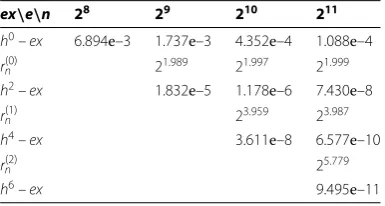
Table 2 The numerical results fort= 0.984375
ex\e\n 28 29 210 211
h0–ex 6.894e–3 1.737e–3 4.352e–4 1.088e–4
r(0)n 21.989 21.997 21.999
h2–ex 1.832e–5 1.178e–6 7.430e–8
r(1)n 23.959 23.987
h4–ex 3.611e–8 6.577e–10
r(2)n 25.779
h6–ex 9.495e–11
Sinceg(x) = (x– )and (I(g))(t) are non-periodic functions on (, ), we use equations (.). The errors of approximation solution are listed in Table fort= . by (.) and (.). The numerical results in the table show that
r(nk)≈k+, k= , , ,
which accord with the error expansion of (.) perfectly. Furthermore, the numerical re-sults in the table also display the fact that a higher convergence order can be got by the extrapolation method.
Example . Calculate the hyper-singular integral
I(g)(t) =
–
g(x)
|x–t|dx, g(x) =e
x, (.)
where the exact solution is
I(g)(t) =et
∞
k=
k!k
(– –t)k+ ( –t)k+ etln| +t|+ln| –t|.
The numerical results are listed in Table based on the quadrature formulas (.) and the Romberg extrapolation att= ..
Note that the convergence order of numerical solutions can be improved by an extrapo-lation method. From the numerical results in Table , we haverk
n≈k+(k= , , ), which
agrees with the rules of (.) and (.).
Example . Calculate the hyper-singular integral
I(g)(t) =
g(x)
(x–t)dx, g(x) =x
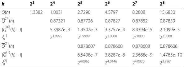
[image:12.595.202.395.228.331.2]Table 3 The numerical results fort= 0.25
h 23 24 25 26 27 28
Q(h) 1.3382 1.8031 2.7290 4.5797 8.2808 15.6830
Q(0)(h) 0.87321 0.87726 0.87827 0.87852 0.87859
|Q(0)(h) –I| 5.3987e–3 1.3502e–3 3.3757e–4 8.4394e–5 2.1099e–5
r(1)n 21.9995 21.9999 22.0000 22.0000 22.0000
Q(1)(h) 0.878607 0.878608 0.878608 0.878608
|Q(1)(h) –I| 6.5498e–7 3.8287e–8 2.3688e–9 1.4785e–10
[image:13.595.141.458.237.325.2]r(2)n 24.0965 24.0146 24.0020 23.9961
Table 4 The numerical results fort= 0.25
ex\e\n 23 24 25 26 27 28 29
h0–ex 3.600e–2 1.240e–2 4.286e–3 1.490e–3 5.202e–4 1.823e–4 6.405e–5 r(0)n 21.5379 21.5326 21.5246 21.5178 21.5128 21.5091
h2–ex 5.107e–4 1.514e–4 3.955e–5 9.998e–6 2.506e–6 6.271e–7
r(1)n 21.7538 21.9368 21.9840 21.9960 21.9990
h4–ex 3.168e–5 2.262e–6 1.469e–7 9.272e–9 5.810e–10
r(2)n 23.8081 23.9447 23.9855 23.9963
where the exact solution is
I(g)(t) = t
– t+ t+ t+ t+ (t– ) + t
ln
–t t
, t∈(, ).
We get the quadrature formulasQh=h
n–
k=g((
+k)h)/((
+k)h–t)
from rules (.)
and extrapolations (.) for this example. We have the numerical results listed in Table for (.) by using the rules (.) and (.) att= . withα= – andIis the Hadamard part of the example.
Clearly, the numerical results in Table imply that
r(nk)≈k, k= , , which meet equation (.).
Example . Calculate the hyper-singular integral with the fractional order singularity
I(g)(t) =
g(x)
|x–t|dx, g(x) = (x– )
, (.)
where the exact solution is
I(g)(t) = –.
y– y+ y–
√y +y
– y+ y– √
–y
.
The numerical results for (.) att= . are listed in Table by (.) and a Richardson extrapolation. Sinceg(i)(x) = fori= , , . . . , the error analysis of equation (.) is
En(h) = m+
k=
akhk+bh.+O
Figure 1 Nonlinear regression analysis att= 0.25.Note that the order of convergence matches the error analysis and the order is clearly improved by using an extrapolation.
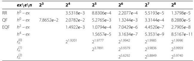
Table 5 The numerical results of QF, EQF, and RR witht= 0.25
ex\e\n 23 24 25 26 27 28
RR h0–ex 3.5318e–3 8.8306e–4 2.2077e–4 5.5193e–5 1.3798e–5 QF h0–ex 7.8652e–2 2.0782e–2 5.2765e–3 1.3244e–3 3.3144e–4 8.2880e–5 EQF h2–ex 1.4922e–3 1.0794e–4 7.0429e–6 4.4520e–7 2.7905e–8
h4–ex 1.5657e–5 3.1634e–7 5.3531e–9 8.5167e–11
r(0)n 21.9201 21.9777 21.9942 21.9985 21.9996
r(1)n 23.7891 23.9379 23.9836 23.9959
r(2)n 25.6292 25.8849 25.9740
whereakandbare constants, which are independent ofh. The numerical results of Ta-ble also indicate that
r()n ., rn(), r()n ,
which coincide with (.) perfectly.
The nonlinear regression analysis shows thate()n = .h.after the fractional order
extrapolation, whilee()n = .h.ande()n = .h.are after the integer order
extrap-olation. We show this nonlinear regression analysis result graphically on Figure .
Example . Calculate the hyper-singular integral of Example . withg(x) =x+ and the exact value of this finite-part integral is
I(g)(t) = t+ t+ +
t+
t(t– )+ t ln –t
t .
[image:14.595.134.459.330.433.2]The numerical results in the table display the fact that EQF has a high accuracy com-pared with the method of RR and QF. Furthermore,
r(nk)≈k+, k= , , ,
which accord with the error expansion of (.) perfectly. The ratelog(rnk) shows that EQF has fourth and sixth order accuracy ask= andk= , respectively.
In a consideration of the non-periodic functions g(x) of all the numerical examples above, we can periodize the functions by asinp transformation [] to take away some terms of the error expansions. By utilizing the extrapolation method, we can get numeri-cal solutions with higher convergence order from (.), (.), and (.), respectively.
5 Conclusion
From the above results in this paper, we draw conclusions as follows: According to the quadrature formulas to calculate hyper-singular integrals, the algorithms of modified trapezoidal formulas have a low cost for real world problems compared with some other methods, such as the Gaussian method [, , ] and the Newton-Cotes method [– ]. The rules can be calculated in a fairly straightforward way, without the need to calcu-late any weight. The accuracy order of the algorithms is very high. Finally, the numerical experiments match with the error analyses. These excellent numerical results show the significance of the quadrature formulas proposed in this paper.
Competing interests
The authors declare that they have no competing interests.
Authors’ contributions
The authors declare that the work was realized in collaboration with the same responsibility. All authors read and approved the final manuscript.
Acknowledgements
The authors would like to thank the editor and referees for useful comments and suggestions. The authors of this paper were supported by the National Science Foundation of China (11371079).
Received: 1 July 2015 Accepted: 21 December 2015 References
1. Lifanov, IK, Poltavskii, LN, Vainikko, GM: Hyper-Singular Integral Equations and Their Applications. CRC Press, Boca Raton (2004)
2. Monegato, G, Lyness, JN: The Euler-Maclaurin expansion and finite-part integrals. Numer. Math.81, 273-291 (1998) 3. de Lacerda, LA, Wrobel, LC: Hyper-singular boundary integral equation for axisymmetric elasticity. Int. J. Numer.
Methods Eng.52, 1337-1354 (2001)
4. Cheng, M: Hyper-singular integral operators on modulation spaces for 0 <p< 1. J. Inequal. Appl.2012, 165 (2012) 5. Chen, JT, Kuo, SR, Lin, JH: Analytical study and numerical experiments for degenerate scale problems in the boundary
element method for two-dimensional elasticity. Int. J. Numer. Methods Eng.54, 1669-1681 (2002)
6. Amann, D, Blaszczyk, A, Of, G, Steinbach, O: Simulation of floating potentials in industrial applications by boundary element methods. J. Math. Ind.4, Article 13 (2014)
7. Kim, P, Choi, UJ: Two trigonometric quadrature formulae for evaluating hyper-singular integrals. Int. J. Numer. Methods Eng.56, 469-486 (2003)
8. Huang, J, Wang, Z, Zhu, R: Asymptotic error expansions for hyper-singular integrals. Adv. Comput. Math.38, 257-279 (2013)
9. Kabir, H, Madenci, E, Ortega, A: Numerical solution of integral equations with logarithmic-, Cauchy- and Hadamard-type singularities. Int. J. Numer. Methods Eng.41, 617-638 (1998)
10. Hui, CY, Shia, D: Evaluations of hyper-singular integrals using Gaussian quadrature. Int. J. Numer. Methods Eng.44, 205-214 (1999)
11. Chen, YZ: Hyper-singular integral equation method for three-dimensional crack problem in shear mode. Commun. Numer. Methods Eng.20, 441-454 (2004)
13. Alpert, BK: Hybrid Gauss-trapezoidal quadrature rules. SIAM J. Sci. Comput.20, 1551-1584 (1999)
14. Cialdea, A, Leonessa, V, Malaspina, A: Integral representations for solutions of some BVPs for the Lamé system in multiply connected domains. Bound. Value Probl.2011, 53 (2011)
15. R ˘apeanu, E, Carabineanu, A: A Green function approach for the investigation of the incompressible flow past an oscillatory thin hydrofoil including floor effects. Bound. Value Probl.2014, 104 (2014)
16. Li, J, Yu, D: A rectangle rule for the computation of hyper-singular integral. IOP Conf. Ser., Mater. Sci. Eng.10, 012115 (2010)
17. Monegato, G: Numerical evaluation of hyper-singular integrals. J. Comput. Appl. Math.50, 9-31 (1994) 18. Paget, DF: The numerical evaluation of Hadamard finite-part integrals. Numer. Math.36, 447-453 (1980/81) 19. Du, QK: Evaluations of certain hyper-singular integrals on interval. Int. J. Numer. Methods Eng.51, 1195-1210 (2001) 20. Linz, P: On the approximate computation of certain strongly singular integrals. Computing35, 345-353 (1985) 21. Wu, JM, Lü, Y: A superconvergence result for the second-order Newton-Cotes formula for certain finite-part integrals.
IMA J. Numer. Anal.25, 253-263 (2005)