A Viterbi tracker for local features

A Viterbi Tracker for Local Features

Gary Baugh

and Anil Kokaram

Trinity College Dublin, Dublin 2, Ireland.

_{[email protected],}

_{[email protected]}

ABSTRACT

The long term tracking of sparse local features in an image is important for many applications including camera calibration for stereo applications, camera or global motion estimation and people surveillance. The majority of existing tracking frameworks are based on some kind of prediction/correction idea e.g. KLT and Particle Filters. However, given a careful selection of interest points throughout the sequence, the problem of tracking can be solved with the Viterbi algorithm. This work introduces a novel approach to interest point selection for tracking using the Mean Shift algorithm over short time windows. The resulting points are then articulated within a Viterbi algorithm for creating very long term tracking data. The tracks are shown to be more accurate than traditional KLT implementations and also do not suffer from accumulation of error with time.

1. INTRODUCTION

The tracking of local regions involves matching them in adjacent images throughout a sequence. It is widely accepted that the ideal is to generate long contiguous tracks. Such tracking data can then be used for camera calibration, surveillance,1 and sparse to fine motion estimation or segmentation.2 Most point tracking systems are two step: first selecting interest points and then tracking the image material around those points through the sequence. The popular KLT tracker,3 and various Particle trackers4 follow this idea. However, given that it is possible to locate interest points in all the frames of the sequence, it is sensible to constrain a tracker to match only that image material around those detected interest points. Unfortunately, Mikolajczyk5 reports that matching local descriptors is unreliable in terms of recall vs precision, since they are only invariant to a few classes of image transformations (affine for example) encountered in practice. However that experiment was conducted using direct SIFT6 descriptor matching without any constraints about motion or local image appearance information. In this paper we propose a strategy for selecting interest points more suitable for tracking, and we design a more appropriate feature vector using a colour quantisation step. The idea is first to process the existing interest points to generate a set of 3-frame long seed tracks of high confidence, using a low cost process. The tracking problem is then to extend these seeds using the available interest points. That is best solved with the Viterbi algorithm.7 This idea enables long term tracking and also is less prone to accumulation of tracking error with time. We discuss track seed selection first, then present the feature vector design and finally construct the elements of the Viterbi tracker.

2. SELECTING SEED TRACKS

Descriptor Space n n+1 n+2 Descriptor in image Accepted Cluster Rejected Cluster 1 2 3 4 5 6 7 8 7 7 7 7 7 7 7 7 7 7 9 10

Figure 1.Left: Examples of local regions (’dot’ indicate center of region (x y) ) and their corresponding circular neighbour-hoods. Note that only a few regions are shown at selected scales for clarity of illustration. Right: Simplified 2-dimensional illustration of the clustering of the descriptor space for the image subsequence (n, n+ 1, n+ 2). The size of the clusters are determined by the Mean Shift kernel bandwidth (radius of circle). Accepted clusters (1,3,8,9) contain only a single descriptor from all three imagesn, n+ 1,andn+ 2.

n n+1 n+2 n+3 n+4 n+5 n+6

p2

n

p1

n

p1

n+ 6 p2

n+ 6 p3

n

p3

n+ 2 p4

n+ 2

p4

n+ 6 p5

n+ 4 p5_{n+ 6}

Frame window

Unconnected

p® ¯

In track with state vector Local Region P1 n P 2 n P 3 n Track P4 n P 5 n

Figure 2. Example of a trellis for local region tracking. Each node (circle) represents a feature vectorpα_β for a local region, where βis the image at which the region was detected, and αis the track index. Three overlapping frame windows are shown (n, n+ 1, n+ 2),(n+ 2, n+ 3, n+ 4), and (n+ 4, n+ 5, n+ 6).

Seed tracks are generated initially using frame windows of 3 frames with an overlap of 1 frame. Hence the first two frame windows have image indexes of (1,2,3), and (3,4,5). Where the end of one 3 frame path coincides with the start of the next 3 frame path, the paths are collated into a new longer seed path. This is performed over the entire sequence resulting in seed paths of arbitrary lengths. The next step is to extend the paths using more region information as well as motion constraints. The appearance information is presented below.

3. THE FEATURE VECTOR AND TRACKING PRELIMINARIES

In order to describe the local region appearance, a feature vector p= (x s g c) is associated with each interest point. The vector contains the position of the point x = (x, y)T, scale and dominant orientation from the SIFT descriptor, s= (σ o)T, the 128 point SIFT descriptor itselfgand an adaptively quantised colour vectorc

(discussed later).

Theith track,Pni, that starts in framenis now considered to be a sequence of matched feature vectors pin. Figure 2 shows this situation for the seed tracks from the previous step. The track Pn3, for instance, consists of the feature vectorsp3n, p3n+1, p3n+2

.

3.1 Colour Feature

Colour information should be collected from a region around the interest point. The size of this region should relate somehow to the influence that local image material has on the location of the interest point. The region should be circular (with radiusr) since the detector is based on circularly symmetric gaussians, but depending on the scale the size of the region of interest will change. This relationship is approximatelyr≈11.4811σ+ 2.5419, whereσis the scale of the local region, obtained from the SIFT interest point detector. With this approximation of

Figure 1 (left) shows example local regions and their corresponding neighbourhoods. The colour feature vectorcis a normalized histogram of quantized colours in this neighbourhood, using the YUV colour space. The quantization scheme is non-linear and is discussed next. Note that spatiograms suggested by Birchfield9 could be used as a simplified alternative for creating this vector.

3.1.1 Colour Space Quantization

Figure 1 (left) shows that the neighbourhoods of the local regions overlap substantially and the union of these regions does not cover the whole image. Therefore some colours are more essential than others in representing these regions. By assuming that the colour profile of a local neighbourhood only changes slightly when tracked over a frame window, due to noise and photometric effects, it is sensible to express the region colour using only the colour in the union of all these local regions. Colours outside these regions are irrelevant. Furthermore, assuming that the colour content does not change wildly over a shot, a compact colour representation derived from the first few frames of the sequence would be sufficient to describe colour content over the subsequent frames. This compact represention is achieved by adaptive colour space quantisation.

Colour space quantization is a well researched topic.10–12 There are two steps: palette design, in which a reduced number of palette colours is chosen, and pixel mapping in which each colour pixel is assigned to one of the colours in the palette. In this work we first create palettes for all local neighbourhoods, and then combine them to obtain a global palette, that is used to generate the colour feature vector c. The first 3-frame window is used for quantisation and the resulting quantised colour space is used for the whole sequence.

Local palettes are created by modelling the spatiotemporal volume associated with each 3-frame pathP₁i as a GMM (Gaussian Mixture Model). Because the neighbourhoods associated with each vector inP₁i is variable, a fixed number of pixel samples (5043) are drawn randomly from these regions and that set is used for modelling. This allows a balance in computational load for GMM parameter estimation. The p.d.f. of the colour samples

ci generated from P₁i is therefore as follows.

fi_Ki(ci) = Ki

j=1

Πi_j Nci;θij

(1)

Where θi_j consists of a mean μi_j, covariance Ri_j, mixing weight Πi_j for each of Ki components of the GMM.

These parameters are estimated via Expectation Maximisation using an implementation by Bouman,13 based on ideas from Redner14 and the number of mixture components Ki is estimated using the minimum

descrip-tion length (MDL) criteria of Rissanen.15 The mean components μij, j = 1,2, . . . , Ki of this GMM

con-stitute the local palette for the tracked region along path P₁i. Each track yields Ki mixture components

μi₁,Ri₁,μi₂,Ri₂, . . . ,μi_Ki,Ri_Ki.

The global palette is then extracted from the local palettes by MS clustering ([5 2 2] kernel bandwidth for [Y U V]) of all the local palettes. Each of the resulting G clusters then contains a set of associated mixture components μg_j,Rg_j: j = 1,2, . . . , Kg, where g = 1,2, . . . , G, and Kg is the number local palettes in each

cluster. This MS step in effect shows which of the local palettes are similar. Hence each of these clusters can be represented by a single Gaussian with parameters (μg,Rg) estimated as follows.

μg= 1

Kg Kg

j=1

μg_j, Rg= 1 Kg

Kg

j=1

Rg_j+μg_jμg_jT

−μgμgT (2)

These Gmodels now form the global palette. A global palette colour g is then defined as having parameters

θg= (μg,Rg).

Consider that a pixel site (x, y) has an observed colour vectorξ. An ML estimate for the quantised colourg

to be assigned to that site is generated by choosingg to maximize the log energyeg(ξ) as follows.

eg(ξ) =−ln

(2π)3/2|Rg|1/2

Using all the global palette colours can produce very sparse colour vectors c, since only a few of these colours occur in each local region. To further quantise this space, colours that are not used often from this palette can be discarded, and the retained colour space is used for the final quantised global palette. To do this, each spatiotemporal region associated with a pathP₁i votes for a single colour gi. That colour gi is the colour that

best models the entire patch region, i.e. gi minimises the sum ofeg(ξ) over the whole patch. After all the paths

are processed in this way, all colours which have no votes are discarded. For the example sequences in figure 3, the number of global palette colours are 598,212,235, and 139 respectively.

3.2 Tracking

It is now required to extend the seed paths into long term tracks using the feature vectors associated with each interest point. An adaptation of the Viterbi algorithm7 proposed by Pitie16 is used here. Figure 2 shows an example of a typical initial Viterbi trellis at this stage. The states in the Viterbi algorithm at each frame are all the feature vectors of the detected interest points which include those that are already associated with paths. Note that, it is required to extend the tracks both forward and backward temporally. This bi-directional temporal extension is achieved by first extending all tracks forward in time, and then reversing the Viterbi trellis and extend the tracks forward again. The discussion that follows is therefore applicable to both directions.

The Viterbi algorithm solves the problem of finding the best paths (in a minimum energy sense) connecting the states in the trellis i.e. solving our point tracking problem. The energy associated with each state (or point) in each frame depends both on the feature vector itself as well as an energy associated with the transition between states in consecutive frames. This framework is well understood and more information can be found here.7 The essential requirement however is to define a transition energy between the last state of the trackpi_τ , and theNv

candidate statespv_τ+1 : v= 1,2, . . . , Nv, in imageτ+ 1. HereNv is the number of candidate states in the next

frameτ+ 1. Only feature vectors that are at the start of a track or not associated with any track are considered to be candidates in imageτ+ 1. This transition energy is defined asφi_τ,τ+1pv_τ+1, and is expressed below.

φiτ,τ+1

pvτ+1

=λMpvτ+1; piτ−2,τ−1,τ

+Opvτ+1; piτ−2,τ−1,τ

(4)

Mpv_τ+1; p_τi_{−2,τ−1,τ}is a motion smoothness constraint, andOpv_τ+1; p_τi_{−2,τ−1,τ}is dependent on the colour, scale, and descriptor information of the track. λis a weighting between these energy terms.

3.3 Motion smoothness

When estimating future state spatial locations, it is assumed that tracks in very close proximity to each other change their speeds at the same rate. Hence some spatial smoothness constraint is important. For a trackP_ni, with the feature vector at the end of the track being pi_τ, the last three feature vectors pi_τ−2,pi_τ−1,pi_τ are used to predict the next possible feature vector in imageτ+ 1 to be added to the track. The motion constraint

Mpc_τ+1; pi_{τ−2,τ−1,τ} in (4) penalizes candidate spatial locations xv_τ+1 according to their distance from the predicted spatial location ˜xiτ+1of the trackPni in imageτ+ 1. The predicted spatial location ˜xiτ+1, is estimated using the last known location xiτ, and displacementxiτ−xiτ−1 of trackPni, as follows

˜

xi_τ+1 = xi_τ+Ai_mxi_τ−xi_τ−1+η (5)

Here Ai_m = α

m

x 0

0 αm y

is a displacement magnitude gain matrix, and η ∼ N(0,Ri). The displacement gain

matrix and noise covariance are estimated by using the known seed paths up to the current frame.

A candidate Aj is generated for each path Pnj : j = 1,2, . . . , J that exist over the images τ−2, τ −1, τ,

whereJ is number of such paths. A weighted least square estimate is used that incorporates path information from neighbouring paths as follows.

αjx=

k

w2_(j,k)|xk_τ−2−x_τk₋₁||xk_τ−1−xk_τ|

k

w₍2_j,k)|xk_τ−2−xk_τ−1|2

, αjy=

k

w2_(j,k)|y_τk₋₂−y_τk₋₁||y_τk₋₁−y_τk|

k

w₍2_j,k)|yk_τ−2−y_τk₋₁|2

Wherew₍j,k)=√₂1πσsexp −0.5 δT_δ

2σ2_s

, δ=xk_τ−2+xk_τ−1+xk_τ/3− xj_τ−2+xj_τ−1+xj_τ

/3, andk= 1,2, . . . , J. A constant spatial variance σs= 50 is used.

Every track is now associated with a particularAi_mby choosing thatAj from amongst the candidate set that

minimises the prediction error defined as follows.

j=|xjτ−1−xjτ| −Aj|xjτ−2−xjτ−1| (7)

The covariance matrix of those prediction errors is used as an estimate forRi. Hence the motion smoothness

constraint can be written as

Mpvτ+1; piτ−2,τ−1,τ

=−ln

(2π)|Ri|1/2

−0.5xvτ+1−˜xiτ+1

T

Ri−1xvτ+1−x˜iτ+1

(8)

We are more confident of our motion energy term when a track is moving at a constant speed. Therefore, the motion constraint energy weightingλin (4) is made to be inversely proportional the maximum of the displacement gainsαm_x andαm_y in both spatial dimensions.

3.4 Appearance constraint

The energy associated with the feature vector itself is an appearance energy that enforces the constraint that the appearance of the region in the next frame should be similar to the appearance of the regions along the previous frames in a path. By modelling the scale, SIFT descriptor and colour distributions of the region as a gaussian with varianceRO and meanμ0, the appearance energy is therefore as follows.

Opcτ+1; piτ−2,τ−1,τ

=−ln

(2π)M/2|RO|1/2

−0.5 (κc−μO)TRO−1(κc−μO) (9)

Q=

⎛

⎝gsττ−−22 gsττ−−11 gsττ

cτ−2 cτ−1 cτ

⎞

⎠, μO= 1

3

⎛

⎝gsττ−−22++gsττ−−11++sgττ

cτ−2+cτ−1+cτ

⎞

⎠, RO =1

3QQ

T _−μ OμOT

Where the parametersRO and mean μ0 are measured using the values of the feature vector along the path in the three previous frames, and κv =svτ+1T gvτ+1T cvτ+1T

T

, is the scale, SIFT descriptor, and colour vectors for the candidate statepv_τ+1. The off-diagonal elements of theM ×M covariance matrixRO are set to zero,

assuming independence amongst the rows ofQ.

4. PERFORMANCE EVALUATION

The performance of Viterbi tracker is compared to a standard KLT tracker implementation17derived from the work of.18, 19 For the KLT tracker, the maximum number of features to track must be specified. Therefore, we use the total number of tracks in the first frame of the Viterbi tracker to specify the maximum number of track for the KLT tracker. So both trackers start with the same number of tracked features. Only the tracks from the first frame of each sequence are used for analysis since they potentially exist over the entire sequence. Comparing these tracks can reveal how tracking errors are propagated through time.

One natural sequence and three synthetic sequences of known affine transformations are used for testing and the start frame of each are shown in figure 3.

Two criteria are used to assess tracking performance in the synthetic sequences. The synthetic sequences are generated using known affine transformations zoom, rotation and translation. Then the spatial positions of the tracks xi_n, reported by both trackers are used to calculate a least squares estimate for the affine transformation parameters. The error in estimation provides one measure of the usefulness of the tracks. The second criterion used is to compare the actual expected spatial position of the tracks at thenth frame given their starting position

Figure 3. First frames from the graveyard(1920×1080), clock(475×475), house(419×419), and dock (416×220) sequences used to compare the performance of the KLT and Viterbi trackers. The clock, house, and dock sequences are each 251 frames synthesized with known affine transformations. The graveyard sequence is 19 frames of a natural outdoor scene.

Parameter End point KLT Viterbi KLT Viterbi mean 0.79 0.04 2.22 0.77 std 0.28 0.01 3.24 0.32

Table 1. The overall parameter estimation and end point percentage errors for all three synthetic sequence.

The parameters used for the synthetic sequences (zoom zn, rotational θn, and translational tn) vary with

time and are shown below.

zn= 0.5{1 +zmin+ (1−zmin)cos(ωΔt(n−1))} (10)

θn= (n−1)ωΔt, tn =sin(ωΔ₀t(n−1)) 0₀dmax (11)

Wherezmin = 0.4 is the minimum zoom level, dmax = (50 0)T is the maximum translation, Δt = 40ms, and ω= 0.6283rad/s.

Each sequence exhibits just one effect i.e. zoom for theclock, rotation for thehouseand translation for the

dock. The corresponding least squares estimates are ˆzn, θˆn, ˆtn and are derived in the usual manner using all

the estimated feature point locations in a frame.

The percentage errors in the estimation of the zoom, rotation, and translation parameters at thenth frame are defined asz,zminn ,θn, andtn.

4.1 Results and Discussion

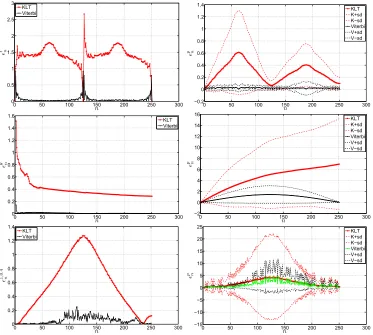
Figure 4 shows performance for both trackers using the synthetic sequences. The left column plots the percentage error in estimating the global motion parameters for both trackers. In red is the KLT while in black is the tracker presented here. The right column shows the corresponding percentage end point error for each tracker. An overall summary of the performance of the trackers for all three sequences in shown in table 1. These results show that the Viterbi tracker produces much more accurate tracks in general. Lower end point errors are achieved, with relatively small standard deviation across the image. This indicates that the Viterbi tracks are more dependable locally. Considering the rotational sequence (house), the standard deviation of the end point error for the KLT tracker increases with time. This indicates that there is significant track drift for this tracker when the sequence undergoes rotational transformation. The zoom sequence is the most challenging to track because of the significant loss of local features due to scale change with time. In the experiment the clock sequence was zoomed from 100% to 40% and back to 100%. For this sequence, the KLT tracker had a mean end point error of 1.92% with a std (standard deviation) of 0.82%. The corresponding error for the Viterbi tracker was 1.38% with a std of 0.08%. This is a substantial improvement. In addition, the average length of tracks for each sequence shown in figure 3 using the KLT was 10, 68, 251, and 95 respectively while for the Viterbi tracker it was 9, 33, 132, and 179. Even though the KLT tracker maintains much longer tracks for the zoom (clock) and rotation (house) sequences, the parameter and end point errors are relatively large compared to the Viterbi tracker. In the case of the zoom sequence, where there are rapid local image deformations, the average track lengths are expected to be shorter.

0 50 100 150 200 250 300 0 0.5 1 1.5 2 2.5 3 t n n KLT Viterbi

0 50 100 150 200 250 300

−0.2 0 0.2 0.4 0.6 0.8 1 1.2 1.4 p n n KLT K+sd K−sd Viterbi V+sd V−sd

0 50 100 150 200 250 300

0 0.2 0.4 0.6 0.8 1 1.2 1.4 1.6 θ n n KLT Viterbi

0 50 100 150 200 250 300

−2 0 2 4 6 8 10 12 14 16 p n n KLT K+sd K−sd Viterbi V+sd V−sd

0 50 100 150 200 250 300

0 0.2 0.4 0.6 0.8 1 1.2 1.4 z, 0 . 4 n n KLT Viterbi

0 50 100 150 200 250 300

−15 −10 −5 0 5 10 15 20 25 p n n KLT K+sd K−sd Viterbi V+sd V−sd

Figure 4. The left column shows the global performances of the trackers for the translational, rotational, and zoom sequences. The corresponding local performances (endpoint error) for these sequences is shown in the right column, where p_n± one standard deviation is shown as K+sd and K-sd, V+sd and V-sd, for the KLT and Viterbi trackers respectively.

Figure 5. The tracks up to the 6st frame of the graveyard sequence for selected cropped areas. The top and bottom rows are the tracks produced by the KLT and Viterbi tracker respectively. Column 1: Trees - strong corner features. Column 2: Tomb - edges in direction of motion and flat image regions. Column 3: Pavement - mostly flat image region. Column 4: Grass - repetitive texture.

lost them on the smooth surface. Birchfield20 identified that repetitive textures can cause individual features to be distracted by similar nearby patterns in a standard KLT tracker. This phenomenon is observed in the grass area for the KLT tracker but not for the Viterbi tracker. The Viterbi tracker produces more tracks for the grass since more interest points can be found this highly textured region. Where there are very strong corner feature like the tree area, the performance of both trackers is roughly the same.

5. CONCLUSION

A new algorithm has been presented for tracking feature points over time. It is deterministic and exploits the use of a novel feature selection process based on temporal pre-selection and colour quantisation. The performance is more reliable than.17 It is encouraging that the system presented does not suffer from the drift issues as much as the prediction/correction process of the KLT. We expect this is due to the use of candidate tracking points instead of continuous tracking. Future work will consider what aspects of this process bring to the tracking problem. By changing the feature point detector to a Harris corner detector for instance, we would be able to assess the impact of the detector with respect to the KLT. It is important to recognise that the Viterbi process itself is little more than a KLT with a restriction to search at candidate points only. Thus the advantages of this process only express when the candidates are unique and considerably fewer than the corners that might be used in the KLT. In the results shown here there were on average 1747 feature per frame in the KLT as compared to 1574 in our system. We shall explore these issues in future work.

ACKNOWLEDGMENTS

This work was supported by the Science Foundation Ireland research frontiers programmme: SFI-RFP06-06RFPENE004 and by the EU FP7 Project i3DPost Contract Number 211471.

REFERENCES

[1] Baugh, G. and Kokaram, A., “Feature-based object modelling for visual surveillance,” in [Image Processing, 2008. ICIP 2008. 15th IEEE International Conference on], 1352–1355 (2008).

[2] Pundlik, S. J. and Birchfield, S. T., “Real-time motion segmentation of sparse feature points at any speed,”

Systems, Man, and Cybernetics, Part B: Cybernetics, IEEE Transactions on 38(3), 731–742 (2008). [3] Baker, S. and Matthews, I., “Lucas-kanade 20 years on: A unifying framework,”International Journal of

Computer Vision56, 221–255 (2004).

[4] Arnaud, E. and Memin, E., “Partial linear gaussian models for tracking in image sequences using sequential monte carlo methods,”International Journal of Computer Vision74(1), 75–102 (2007).

[5] Mikolajczyk, K. and Schmid, C., “A performance evaluation of local descriptors,” Pattern Analysis and Machine Intelligence, IEEE Transactions on27(10), 1615–1630 (2005).

[6] Lowe, D., “Distinctive image features from scale-invariant keypoints,” International Journal of Computer Vision 20, 91–110 (2003).

[7] Forney, G. D., J., “The viterbi algorithm,”Proceedings of the IEEE61(3), 268–278 (1973).

[8] Pooransingh, A., Radix, C. A., and Kokaram, A., “The path assigned mean shift algorithm: A new fast mean shift implementation for colour image segmentation,” in [Image Processing, 2008. ICIP 2008. 15th IEEE International Conference on], 597–600 (2008).

[9] Birchfield, S. T. and Sriram, R., “Spatiograms versus histograms for region-based tracking,” in [Computer Vision and Pattern Recognition, 2005. CVPR 2005. IEEE Computer Society Conference on],2, 1158–1163 vol. 2 (2005).

[10] Scheunders, P., “A comparison of clustering algorithms applied to color image quantization,”Pattern Recog-nition Letters18(11-13), 1379–1384 (1997). doi: DOI: 10.1016/S0167-8655(97)00116-5.

[11] Papamarkos, N., Atsalakis, A. E., and Strouthopoulos, C. P., “Adaptive color reduction,”Systems, Man, and Cybernetics, Part B: Cybernetics, IEEE Transactions on32(1), 44–56 (2002).

[12] Hsieh, I.-S. and Fan, K.-C., “An adaptive clustering algorithm for color quantization,”Pattern Recognition Letters21(4), 337–346 (2000). doi: DOI: 10.1016/S0167-8655(99)00165-8.

[14] Redner, R. A. and Walker, H. F., “Mixture densities, maximum likelihood and the em algorithm,”SIAM Review26(2), 195–239 (1984).

[15] Rissanen, J., “A universal prior for integers and estimation by minimum description length,” Annals of Statistics11(2), 416–431 (1983).

[16] Pitie, F., Berrani, S. A., Kokaram, A., and Dahyot, R., “Off-line multiple object tracking using candidate selection and the viterbi algorithm,” in [Image Processing, 2005. ICIP 2005. IEEE International Conference on],3, III–109–12 (2005).

[17] Birchfield, S. T., “Klt: An implementation of the kanade-lucas-tomasi feature tracker,” (2007).

[18] Tomasi, C. and Kanade, T., “Shape and motion from image streams: a factorization method - part 3 detection and tracking of point features,” tech. rep., Computer Science Department (April 1991).

[19] Jianbo, S. and Tomasi, C., “Good features to track,” in [Computer Vision and Pattern Recognition, 1994. Proceedings CVPR ’94., 1994 IEEE Computer Society Conference on], 593–600 (1994).