Impacts of Policies on Poverty Basic Poverty Measures

Impacts of Policies on Poverty. Basic

Poverty Measures

Bellù, Lorenzo Giovanni and Liberati, Paolo

Food and Agriculture Organization of the United Nations (FAO)

AN ALYTI CAL TOOLS

Impacts of Policies on

Poverty

Basic Poverty Measures

Be llù , Lor en zo Giova n n i,1 Libe r a t i, Pa olo 2

1

Agr icult ure Policy Support Service, Policy Assist ance Division, FAO 2

Universit y of Urbino, " Car lo Bo" , I nst it ut e of Econom ics, Urbino, I t aly

Resour ces f or policy m ak in g

EASYPol Module ₀₀₇

FOOD AN D AGRI CULTURE ORGAN I ZATI ON OF TH E UN I TED NATI ON S, FAO

About EASYPol

EASYPol is a m ult ilingual reposit ory of freely dow nloadable resources for policy m aking in agricult ur e, rural developm ent and food securit y. The EASYPol hom e page is av ailable at:

The designat ions em ployed and t he pr esent at ion of t he m at er ial in t his infor m at ion pr oduct do not im ply t he expression of any opinion w hat soever on t he par t of t he Food and Agr icult ur e Or ganizat ion of t he Unit ed Nat ions concer ning t he legal st at us of any count r y, t er r it ory, cit y or ar ea or of its aut hor it ies, or concer ning t he delim it at ion of it s fr ont ier s or boundar ies.

I m pact s of Policies on Povert y

Basic Pover t y Measures

Table of Cont ent s

1 Sum m ary ………. 1

2 I nt roduct ion ……… 1

3 Concept ual background ……… 1

3.1 The head- count rat io ( HC) ... 2

3.2 The Pov ert y Gap ( PG) ... 3

4 A st ep- by- st ep procedure t o build HC and PG ………..4

4.1 A st ep- by- st ep procedur e t o calculat e HC ... 4

4.2 A st ep- by- st ep procedur e t o calculat e PG ... 5

5 A num erical exam ple of how t o calculat e HC and PG ……… 6

5.1 An exam ple of how t o calculat e HC _{... 6}

5.2 An exam ple of how t o calculat e PG ... 7

6 On t he propert ies of HC and PG ……… 8

6.1 The m ain propert ies of HC ... 8

6.2 The m ain propert ies of PG ... 10

7 A synt hesis ………..11

8 Readers’ not es ………. 12

8.1 Tim e requirem ent s ... 12

8.2 Frequent ly ask ed quest ions ... 12

8.3 EASYPol links ... 12

1 SUM M ARY

This module describes two of the most commonly used poverty measures in applied policy works, i.e., the headcount ratio (HR) and the poverty gap (PG) ratio. These are basic poverty indicators used to investigate impacts of public policies on poverty. After providing a conceptual background to HR and PG, this module describes step-by-step procedures and provides numerical examples to calculate these measures. In addition, advantages and shortcomings of these measures are discussed, and their explanatory power is investigated.

2 I N TRODUCTI ON

Obj e ct ive s

Poverty measurement is essential to implement effective policies to fight poverty and to evaluate the poverty impacts of other policies. The aim of this module is to illustrate two simple approaches to poverty measurement. In particular, this module deals with how to build the headcount ratio and the poverty gapratio.

Ta r g e t a u d ie n ce

This module targets current or future policy analysts who want to assess and/or monitor the impact of policies on poverty. In addition, academics, officers in ministries and other professionals can make use of this material for their work. Furthermore, students interested in poverty issues may find this material relevant for their studies.

Re qu ir e d b a ck g r ou n d

The trainer should verify that the audience is familiar with the concept of income distribution and with the concept of poverty, especially with the poverty line definition. Basic knowledge of mathematics and statistics is required.

A complete set links of other related EASYPol modules are included at the end of this module. However, readers will also find links to related material throughout the text where relevant1

3 CON CEPTUAL BACKGROUN D .

Poverty measurement requires that relevant characteristics of poor people be aggregated in a given way. In poverty analysis this problem is known as the «aggregation

1

EASYPol hyperlinks are shown in blue, as follows: a) training paths are shown in u nde r lin e d bold font;

b) other EASYPol modules or complementary EASYPol materials are in bold un de r lin e d it a lics; c) links to the glossary are in bold; and

EASYPol Module 007

Analyt ical Tools

2

problem», i.e. how to pass from the identification of poverty to the measurement of

poverty2.

Measuring poverty goes back a long way in history. Consequently, we have many available poverty indices. One of the main issues in poverty analysis, therefore, is which of the poverty indices do we choose? The best way of selecting a poverty index is to investigate whether it satisfies some of the desirable properties. For example, should a poverty index increase if poverty increases? Should a poverty index be sensible to the number of poor people or rather to the level of their incomes with respect to the poverty line? 3

In poverty measurement there is a basic distinction between ad hoc measures and

axiomatic measures. The first set of measures, widely used until the axiomatic

approach was developed by Sen, 1976, lacks a theoretical derivation. Whereas, the second set of measures is explicitly based on a set of desirable properties that a poverty index should respect (axioms). In addition, a third set of measures, which derived directly from the stochastic dominance literature, is based on the dominance of either Lorenz Curves or Generalized Lorenz Curves4_.

The availability of so many indices has made poverty measurement a field that has generally been fraught with disagreement and difficulties. This is the reason why «the» measure of poverty does not exist. Rather, there are many possible ways of measuring poverty.

We will now look at the simplest ad hoc _{poverty measures. Two widely used poverty}

indexes belonging to this category are:

 The head-count ratio (HC);

 The poverty gap (PG).

3 .1 Th e h e a d- coun t r a t io ( H C)

The headcount ratio (HC) is the simplest way of measuring poverty. It gives the percentage of population which is not above the poverty line. It can be formally defined as follows:

[1]

N P

HC =

2

On the identification of poverty see the EASYPol Modules 005 and 006 respectively: I m pa ct s of Policie s on Pove r t y : Absolu t e Pove r t y Lin es, I m pa ct s of Policie s on Pove r t y : Re la t ive Pove r t y Lin e s. _{On the conceptual difference between identification and aggregation, see Sen, 1997, Chapter A.6.} 3

This discussion is addressed in the EASYPol Module 008: I m pa ct s of Policie s on Pove r t y : Ax iom s for Pove r t y M e a su r e m en t.

4

where P is the number of poor people (those below a poverty line z) and n is total population5.

It is worth noting that HC is directly related to the Cumulative Distribution Function (CDF) F(y). The latter, by definition, gives the percentage of population below a given income level. At income level z, the corresponding value of the CDF illustrates the percentage of the poor population, i.e. HC = F(z).

There are uncountable examples of the use of the headcount ratio in empirical works. Almost any applied policy work on poverty uses this very simple poverty measurement. Just to quote some examples, Deaton, 1997, reports headcount ratio for Côte d’Ivoire in the period 1985-1988, showing that poverty hit 30 per cent of the population in 1985 and about 46 per cent in 1988. The author also reports analogous figures for South Africa in 1993, showing that Blacks were more in poverty than Whites (about 32 per cent and almost zero per cent, respectively).

3 .2 Th e Pover t y Ga p ( PG)

For any individual, the poverty gap may be defined as the distance between the poverty line z and his/her own income y. Aggregating individual poverty gaps for all poor individuals, gives the aggregate poverty gap:

[2]

∑

(

)

= − = P i i y z PG 1

where P is the number of poor individuals (and not the size of total population!). A refined version of the poverty gap normalises expression [2] over the maximum amount of money that would be needed to wipe out poverty. This last amount is given by the product between the number of poor individuals P and the poverty line z.

The intuition is simple. As z represents the minimum individual income for which an individual is not considered poor, the product of this income with the number of poor individuals P gives the amount of money that is necessary to eradicate poverty.

According to this definition, we have a normalised version of the poverty gap:

[3]

∑

=      − = P i i Pz y z PG 1 5

An alternative analytical expression is

(

)

∑

EASYPol Module 007

Analyt ical Tools

4

In turn, expression [3] may be restated in another way. As P and z are constants under the summation sign, we can rewrite:

[4]

z y Pz Y Pz Pz Pz

y z

PG P P

P

i

i _{= − = −}

   

  −

=

∑

=

1 1

where YP is the total income of poor individuals, while yp is the mean income of the poor. Expression [4] may be defined as «the percentage of average income of the poor that falls short of the poverty line».

The same observation made for the headcount ratio holds for the poverty gap. Headcount ratio and poverty gap are indeed almost universally reported as the two basic poverty measurements, for both temporal and cross-sectional analysis and in both developed and less developed countries. This is the case, for example, for the Jamaica Food Stamp Programme6, for the poverty analysis on the Russian Federation7 and for the poverty analysis of Papua New Guinea8. A poverty gap of 0.142 in 1988 recorded in Côte d’Ivoire means that the average income of the poor is about 86 per cent of the poverty line (1 – 0.142 = 0.858). The poverty gap in South Africa among Blacks in 1993 is 0.106, which means that the average income of the poor is about 89 per cent of the poverty line (1 – 0.106 = 0.894)9

4 A STEP- BY- STEP PROCEDURE TO BUI LD H C AN D PG .

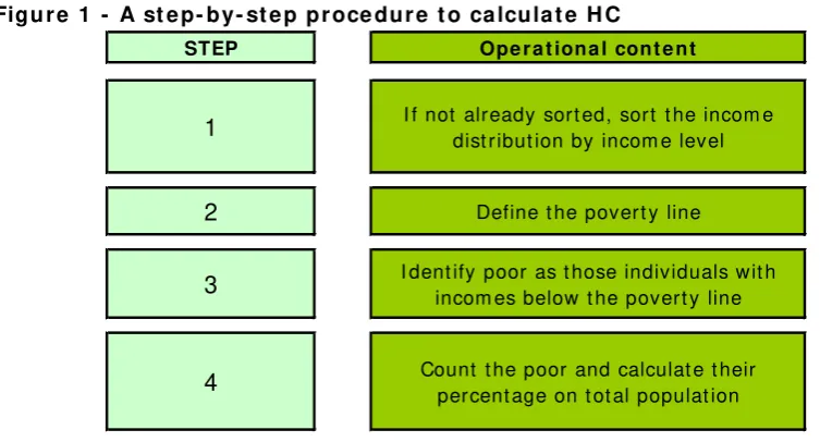
4 .1 A st e p- by- st e p pr oce du r e t o ca lcu la t e H C

Given the restricted number of parameters needed to define HC, the step-by-step procedure is also very simple. Figure 1 illustrates the case.

6

Ezemenari and Subbarao, 1998.

7

Ferrer-i-Carbonell and Van Praag, 2000.

8

Gibson, 1998.

9

Figu r e 1 - A st e p- b y- st e p p r oce du r e t o ca lcu la t e H C

STEP Ope r a t iona l cont e nt

1 I f not already sort ed, sort t he incom e

dist ribut ion by incom e level

2 Define t he povert y line

3 I dent ify poor as t hose individuals wit h _{incom es below t he povert y line}

4 Count t he poor and calculat e t heir _{percent age on t ot al populat ion}

Step 1 is required in order to work with individuals ordered in an ascending level of

income. Income distributions should always be sorted before proceeding to define poverty measurements.

Step 2 is specific to poverty measurement. In what follows, we assume that the poverty

line has already been defined according to either absolute or relative methods10.

Step 3 requires that we focus on individuals with incomes below the poverty line.

Step 4, instead, requires that we count the poor and divide their number by the total

population. This is the headcount ratio.

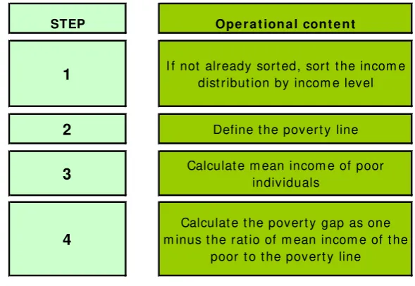
4 .2 A st e p- by- st e p pr oce du r e t o ca lcu la t e PG

Figure 2 illustrates the steps needed to calculate the poverty gap. Step 1 and Step 2 are the same as in the case of HC. According to expression [4], and given the definition of the poverty line, the only parameter that has to be calculated is the mean income of poor individuals (Step 3). By taking 1 minus the ratio of mean income of poor people to the poverty line gives PG (Step 4).

10

EASYPol Module 007

Analyt ical Tools

6

Figu r e 2 - A st e p- b y- st e p p r oce du r e t o ca lcu la t e PG

STEP Ope r a t iona l cont e nt

1 I f not already sort ed, sort t he incom e _{dist ribut ion by incom e level}

2 Define t he povert y line

3 Calculat e m ean incom e of poor _individuals

4

Calculat e t he povert y gap as one m inus t he rat io of m ean incom e of t he

poor t o t he povert y line

5 A N UM ERI CAL EXAM PLE OF H OW TO CALCULATE H C AN D PG

Despite, or because of, their wide uses in empirical work, the way in which these two indexes are built is not usually spelled out. In what follows, therefore, the focus will not be on a real example but on the way to build these indexes starting from a simplified income distribution.

5 .1 An e x a m ple of h ow t o ca lcu la t e H C

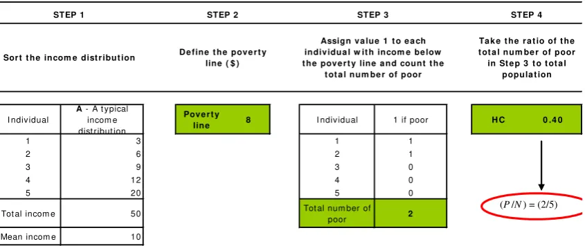
Step 1 – Table 1, below, first illustrates how to calculate HC from a simulated income

distribution. Let us start with an income distribution with five individuals, having a total income equal to 50 currency units and mean income equal to 10 currency units. Sorting the income distribution is the basic task of this step.

Step 2 – Let us also assume that the poverty line is set to 8 currency units (in this case

equal to 80 per cent of mean income in a relativist view).

Step 3 – It is easily seen that poor individuals are two, i.e., those having income below

the poverty line.

Step 4 – As the poor individuals are two, HC can now be calculated by the ratio of the

Ta ble 1 - Th e h e a dcou n t r a t io

I ndividual

A - A t ypical incom e dist ribut ion

Pove r t y

line 8 I ndividual 1 if poor H C 0 .4 0

1 3 1 1

2 6 2 1

3 9 3 0

4 12 4 0

5 20 5 0

Tot al incom e 50 Tot al num ber of

poor 2

Mean incom e 10

Ta k e t he r a t io of t he t ot a l num be r of poor in St e p 3 t o t ot a l

popula t ion STEP 1

Sor t t he incom e dist r ibut ion

STEP 2

D e fine t he pove r t y line ( $ )

STEP 3

Assign va lue 1 t o e a ch individua l w it h incom e be low t he pove r t y line a nd count t he

t ot a l num be r of poor

STEP 4

(P/N) = (2/5)

5 .2 An e x a m ple of h ow t o ca lcu la t e PG

Table 2, below, gives an example of how to calculate the poverty gap, starting from the same initial income distribution as in Table 1.

Step 1 – Let us start again with an income distribution with five individuals, having

total income equal to 50 currency units and mean income equal to 10 currency units. Sorting the income distribution is the basic task of this step.

Step 2 – Let us also assume that the poverty line is again set to 8 currency units (in this

case equal to 80 per cent of mean income in a relativist view).

Step 3 – This step requires that we calculate the average income of poor individuals.

Therefore, incomes of poor individuals must be added and the resulting number divided by the number of poor individuals (two persons in the income distribution).

Step 4 – We are now ready to apply expression [4], giving a PG equal to 0.438. This

EASYPol Module 007

Analyt ical Tools

8

Ta ble 2 - An e x a m p le of h ow t o ca lcu la t e PG

I ndividual

A - A t ypical incom e dist ribut ion

Pove r t y

line 8 I ndividual

I ncom e of poor

individuals PG 0 .4 3 8

1 3 1 3

2 6 2 6

3 9 M e a n incom e

of t he poor 4 .5

4 12

5 20

Tot al incom e 50

Mean incom e 10

Or de r t he incom e dist r ibut ion D e fine t he pove r t y line ( $ )

Ca lcula t e m e a n incom e of poor pe ople ( t hose be low t he

pove r t y line )

Ca lcula t e t he pove r t y ga p STEP 3

STEP 1 STEP 2 STEP 4

6 ON TH E PROPERTI ES OF H C AN D PG

6 .1 Th e m a in pr oper t ies of H C

It is worth discussing some properties of both HC and PG. This discussion will prove useful also in the case of the analysis of other poverty measures. It also introduces the issue of axioms in poverty measurement, i.e. to the set of desirable properties that a poverty measure should have. Simplicity of these measures, as we will show, has some costs in terms of their sensitivity to the change in the income distribution.

The headcount ratio HC has the following properties:

 HC _{has zero as lower limit. It happens when all individuals have an income just}

above the poverty line. In this case, the number of poor is zero and its ratio to total population is also zero.

 HC _{has 1 as upper limit. If everybody is poor, the number of poor people is equal}

to total population.

 HC _{is scale invariant. If all incomes and the poverty line are scaled by the same}

proportional factor α, HC would stay invariant.

 HC _{is translation invariant. If all incomes and the poverty line are increased}

(decreased) by the same absolute amount of money, HC would remain the same. The reason is that HC is independent of the level _{of incomes, as it is only sensitive}

to the number _{of poor.}

poverty line, even though the extreme poor person is now even poorer. Similarly, HC does not increase if a poor individual gives part of his/her income to a rich individual (who is already above the poverty line).

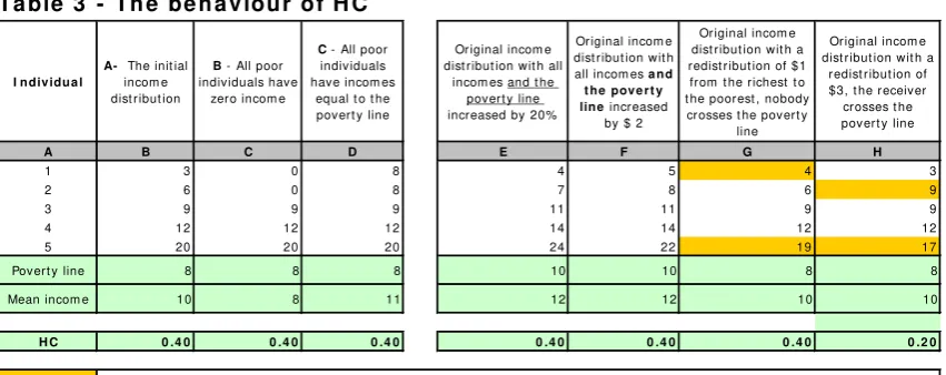
Table 3, below, illustrates, with some examples, the behaviour of HC under alternative hypotheses. Starting from the initial income distribution, it is worth comparing the behaviour of HC with two alternative income distributions: i) the first, income distribution B, is where all poor individuals have zero income; ii) the second, income distribution C, is where all poor individuals have an income equal to the poverty line. In income distribution A, the number of people with an income below the poverty line is 2. Therefore, HC is given by the ratio 2/5, which gives 0.4. This means that 40 per cent of the population is poor. When the incomes of all poor individuals are replaced by zero incomes (income distribution B), the headcount ratio does not change. As in A, there are again two people with incomes below the poverty line. HC is therefore 0.4 also in this case. An analogous line of reasoning can be used for income distribution C. Even though all poor individuals have incomes that are equal to the poverty line, there are again two people who are not above the poverty line. Poverty, as measured by HC, is again 0.4 (columns C and D). This suggests that HC is not sensitive to the depth of poverty. If different distributions give rise to the same number _{of poor, HC will show}

the same value, regardless of the position of individuals with respect to the poverty line. Table 3 also shows that HC is both scale and translation invariant (columns E and F). If

original incomes and the poverty line are increased by 20 per cent, the value of HC

would stay the same. The same happens when both original incomes and the poverty line are increased by the same absolute amount of money (say, 2 currency units). Indeed, columns E and F give the same number for HC, i.e. 0.4.

Columns G and H, instead, show that HC obeys the principle of transfers only when people involved in redistribution cross the poverty line. In the first case (column G), the richest individual gives one unit of income to the poorest individual. But the latter individual still stays below the poverty line. The HC is therefore equal to 0.4. Whereas, in column H redistributing 3 currency units from the richest individual to a poor individual who is lifted out of poverty halves the headcount ratio (from 0.4 to 0.2), as only one person is now in poverty (20 per cent of the total population).

Ta ble 3 - Th e be h a v iou r of H C

I ndividua l

A- The init ial incom e dist ribut ion

B - All poor individuals have

zero incom e

C - All poor individuals have incom es

equal t o t he povert y line

Original incom e dist ribut ion wit h all

incom es and t he povert y line increased by 20%

Original incom e dist ribut ion wit h all incom es a nd t he pove r t y line increased

by $ 2

Original incom e dist ribut ion wit h a redist ribut ion of $1 from t he richest t o t he poorest , nobody crosses t he povert y

line

Original incom e dist ribut ion wit h a

redist ribut ion of $3, t he receiver crosses t he povert y line

A B C D E F G H

1 3 0 8 4 5 4 3

2 6 0 8 7 8 6 9

3 9 9 9 11 11 9 9

4 12 12 12 14 14 12 12

5 20 20 20 24 22 19 17

Povert y line 8 8 8 10 10 8 8

Mean incom e 10 8 11 12 12 10 10

H C 0 .4 0 0 .4 0 0 .4 0 0 .4 0 0 .4 0 0 .4 0 0 .2 0

EASYPol Module 007

Analyt ical Tools

10

6 .2 Th e m a in pr oper t ies of PG

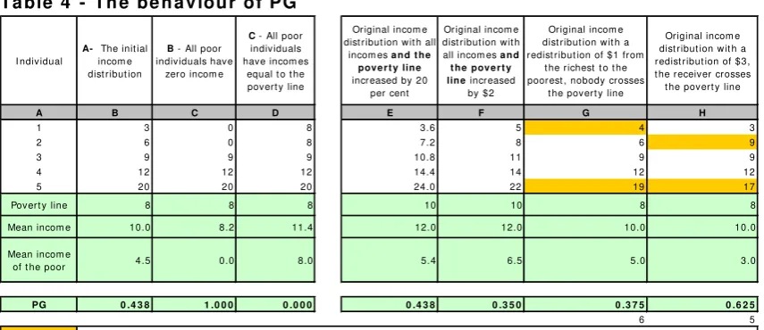
Poverty gap PG has similar properties:

 PG _{has zero as lower limit. When all incomes of poor individuals are equal to the}

poverty line, mean income of the poor and the poverty line itself are equal. The calculated PG is therefore zero.

 PG _{has 1 as the upper limit. When all incomes of poor individuals are equal to}

zero, mean income among the poor is also zero. The calculated PG is therefore 1.

 PG _{is scale invariant. If all incomes and the poverty line are scaled by the same}

proportional factor α, PG would remain the same, as mean income and the poverty line would either increase or decrease by the same percentage.

 PG _{is not translation invariant. If all incomes and the poverty line are increased}

(decreased) by the same amount of money, PG would decrease (increase). Note the difference with HC.

 PG _{satisfies the principle of transfers only in particular cases. If transfers occur}

among poor people, mean income of the poor would not change, and PG would remain the same. PG may also behave in a perverse way, after a progressive transfer, if a poor individual having an income greater than the average income of the poor is lifted out of poverty. In this case, after the poor individual has been lifted out of poverty, the average income of the poor would decrease. This latter effect would increase the poverty gap, even though there are less poor people in poverty. Therefore, depending on the position of the poor individual with respect to mean income of the poor, when he/she is lifted out of poverty the PG measure may either increase or decrease, surely an undesirable feature for a poverty index.

Table 4, below, illustrates the properties of the PG index.

Ta ble 4 - Th e be h a v iou r of PG

I ndividual

A- The init ial incom e dist ribut ion

B - All poor individuals have

zero incom e

C - All poor individuals have incom es

equal t o t he povert y line

Original incom e dist ribut ion wit h all

incom es a nd t he pove r t y line

increased by 20 per cent

Original incom e dist ribut ion wit h all incom es a nd t he pove r t y line increased

by $2

Original incom e dist ribut ion wit h a redist ribut ion of $1 from

t he richest t o t he poorest , nobody crosses

t he povert y line

Original incom e dist ribut ion wit h a redist ribut ion of $3, t he receiver crosses t he povert y line

A B C D E F G H

1 3 0 8 3.6 5 4 3

2 6 0 8 7.2 8 6 9

3 9 9 9 10.8 11 9 9

4 12 12 12 14.4 14 12 12

5 20 20 20 24.0 22 19 17

Povert y line 8 8 8 10 10 8 8

Mean incom e 10.0 8.2 11.4 12.0 12.0 10.0 10.0 Mean incom e

of t he poor 4.5 0.0 8.0 5.4 6.5 5.0 3.0

PG 0 .4 3 8 1 .0 0 0 0 .0 0 0 0 .4 3 8 0 .3 5 0 0 .3 7 5 0 .6 2 5

6 5

Denot es t he individuals involved by t he incom e t ransfer

PG. Whereas, column F reveals that PG is sensitive to absolute translations of the income distributions. By increasing all incomes and the poverty line by 2 currency units, the measured PG is reduced, in the example, to 0.35, as the average income of poor individuals is now higher than in the previous case. In column G, we can see that a

progressive transfer of 1 currency unit reduces the poverty gap (note the difference

with HC). At the same time, it is worth noting the undesirable property of this index, illustrated in column H. After a progressive transfer where the poor individual has been lifted out of poverty, the calculated PG increases from 0.438 to 0.625! This is so because the receiver of the transfer has an initial income of 6 which is above the mean income of the poor (4.5). The opposite would be true if the receiver had an income above the initial mean income of poor individuals. Indeed, the fact that the poverty gap is 0.625 in column H and 0.375 in column G does not mean that eradicating poverty, in

aggregate terms, is easier in the case of column G. If we take the aggregate figure (PG

x poverty line x number of people in poverty) this gives 6 currency units in column G (0.375 x 8 x 2) and 5 currency units in column H (0.625 x 8 x 1).

7 A SYN TH ESI S

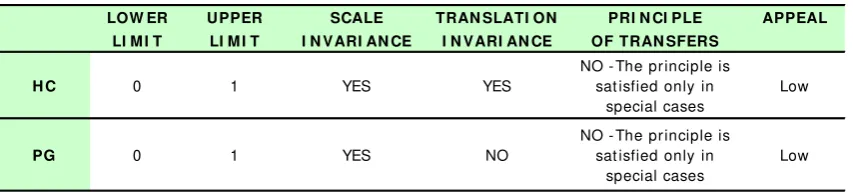
It is worth summarising the main features of HC and PG in table 5.

Ta ble 5 - Th e m a in ch a r a ct e r ist ics of H C a n d PG

LOW ER UPPER SCALE TRAN SLATI ON PRI N CI PLE APPEAL

LI M I T LI M I T I N VARI AN CE I N VARI AN CE OF TRAN SFERS

H C 0 1 YES YES

NO - The principle is sat isfied only in

special cases

Low

PG 0 1 YES NO

NO - The principle is sat isfied only in

special cases

Low

EASYPol Module 007

Analyt ical Tools

12

8 READ ERS’ N OTES

8 .1 Tim e r e qu ir e m en t s

The delivery of this module to an audience already familiar with the definition of poverty both in absolute and relative terms may take about three hours.

8 .2 Fr e qu e nt ly a sk e d qu e st ions

 Is the headcount ratio the simplest way to measure poverty? The answer is yes,

as the headcount ratio only needs to define a poverty line and to count the poor as a proportion of total population. Even though widely used, this measure has serious shortcomings, as it is not very sensitive to changes of the income distribution involving poor individuals.

 How do we remedy the insufficiency of the headcount ratio? In order to give a

more appropriate picture of poverty, poverty measures based on the distance between individual incomes and the poverty line should be used. This is the case of the poverty gap.

 Why are the headcount ratio and the poverty gap so widely used in applied

works? They are easy to calculate and convey an immediate political message:

poor are too many; the distance of the poor from the poverty line is too big. More complicated poverty measures, even though more precise, may be undermined by the difficulty in their interpretation, especially for policy-makers. Nevertheless, we must be aware of the limitations of both HC and PG.

8 .3 EASYPol lin k s

Complementary EASYPol modules are listed here below.

The following modules serve as background material to better understandthe content of the present module

 EASYPol Module 004: I m pa ct s of Policie s on Pov e r t y : The I de finit ion of Pov e r t y

 EASYPol Module 005:I m pa ct s of Policie s on Pov e r t y : Absolut e Pov e r t y Line s

 EASYPol Module 006:I m pa ct s of Policie s on Pov e r t y : Re la t iv e Pov e r t y Line s Furthermore, the modules here below contain more advanced materials on poverty measurement:

 EASYPol Module 008: I m pa ct s of Policie s on Pov e r t y : Ax iom s for Pov e r t y M e a su r e m e nt

 EASYPol Module 009: I m pa ct s of Policie s on Pov e r t y : D ist r ibut iona l Pov e r t y Ga p M e a sur e s

9 REFEREN CES AN D FURTH ER READ I N GS

Deaton A., 1997. The Analysis of Household Surveys, The Johns Hopkins University Press, Baltimore, USA.

Ezemenari K., Subbarao K., 1998. Jamaica’s Food Stamp Program: Impacts on Poverty

and Welfare, Poverty Group, PREM Network, The World Bank, paper presented

at the EDI Workshop, Washington DC, USA, December.

Ferrer-i-Carbonell A., Van Praag B. M. S., 2000. Poverty in the Russian Federation, mimeo, University of Amsterdam, The Netherlands.

Gibson J., 1998. Identifying the Poor for Efficient Targeting: Results for Papua New Guinea, New Zealand Economic Papers, 32, pp. 1-18.

Sen A., 1976. Poverty: An Ordinal Approach to Measurement, Econometrica, 44.