Word Extraction from Speech Recognition using Correlation Coefficients

Word Extraction from Speech Recognition using

Correlation Coefficients

Soumya Sahoo

Assistant Professor C.V Raman College Of

Engineering Bhubaneswar,Odisha

Nilamadhab Das

Assistant Professor C.V Raman College Of

Engineering Bhubaneswar,odisha

Priyambada Sahoo

Assistant Professor C.V Raman College Of

Engineering Bhubaneswar,odisha

ABSTRACT

Speech is the fundamental way of communicating with one another. It simply refers to transmission of messages. In case of speech production the information is transmitted in the form of analog waveform that can be transmitted, recorded or decoded. A number of algorithms for speech recognition have been proposed. In this paper, we have suggested an innovative approach of speech recognition. We have initially stored some voice in the database where the same speaker has told different words. Then we have inputted a sample voice of the same person through the microphone where he is speaking a specific word which is already stored in the database. We have performed the task of similar word recognition by finding the gray scale image and histogram plot of inputted word and finally we have used the correlation coefficient for making comparison between two words.

General Terms

Speech Processing, Word Extraction, Correlation Coefficients.

Keywords

Grayscale Image, RGB, Histogram, Speech Recognition.

1.

INTRODUCTION

Speech is the fundamental analog form of message It is designed to carry sound to aid in hearing. Speech signals, can be converted to an electrical waveform by a microphone. Analog and digital signal processing methods can be used to manipulate these signals. Speech signals can be again converted back to acoustic form by a loudspeaker or a headphone[1]. Speech recognition is a technology that can translate spoken words into text. A speech recognition system can analyze the person's specific voice for recognizing the person’s speech. They can be of two types. Speaker dependent systems and speaker independent systems. Speaker dependent systems uses training whereas speaker independent systems does not use training.

2.

RELATED WORKS

In the year 1995 Speech Recognition using Neural Networks was proposed by Joe Tebelskis where he had examined how artificial neural networks can benefit a large vocabulary, speaker independent, continuous speech recognition system. He explored two different ways to use neural networks for acoustic modeling: prediction and classification. He found that predictive networks yield poor results because of a lack of discrimination, but classification networks gave excellent results. He also verified that, in accordance with theory, the output activations of a classification network form highly accurate estimates of the posterior probabilities P(class|input), and he showed how these can easily be converted to

likelihoods P(input|class) for standard HMM recognition[2] algorithms.

In the year 2003 Chulhee Lee, Donghoon Hyun, Euisun Choi, Jinwook Go, and Chungyong Lee in their paper Optimizing feature extraction for speech recognition had proposed a method to minimize the loss of information during the feature extraction stage in speech recognition by optimizing the parameters of the mel-cepstrum transformation, a transform which is widely used in speech recognition. The mel-cepstrum was obtained by critical band filters whose characteristics play an important role in converting a speech signal into a sequence of vectors. First, they analyze the performance of the mel-cepstrum by changing the parameters of the filters such as shape, center frequency, and bandwidth. Then they proposed an algorithm to optimize the parameters of the filters using the simplex method[3].

In the year 1997 K.Ohtsuki, S. Matsunaga,T.Matsuoka, & S. Furui,in their paper Topic Extraction Based on Continious Speech Recognition in Broadcast News Speech had studied, the extraction of several topic words from broadcast news using continuous speech recognition and found that a combination of multiple topic words represents the contents of the news. They had trained the topic extraction model with five years of newspapers, using the frequency of topic words taken from headlines and words in articles. The degree of relevance between topic words and words in articles is calculated on the basis of statistical measures, i.e., mutual information or the X2 value. In topic extraction experiments for recognized broadcast news speech, they had extracted five topic words using a X2 based model and found that 75% of them agreed with topic words chosen by subjects [4].

3.

AN OVERVIEW OF SPEECH

RECOGNITION

methods used for speech recognition are fast Fourier transform, training using neural network, various statistical techniques etc. But here we have suggested a different approach for speech recognition which is based on image processing.

4.

BASIC IMAGE PROCESSING

CONCEPTS

A digital image is composed of a grid of pixels and stored as an array. A single pixel represents a value of either light intensity or color. Images are processed to obtain information what is visible beyond the given the image’s initial pixel values[6].

4.1

Binary Image

A binary image basically consists of two values that is either zero or one. This type of image is commonly used as a multiplier to mask regions within another image.

4.2

Gray Scale Image

A grayscale digital image is an image in which the value of each pixel is having a single component that is only intensity information. This type of images are also known as black-and-white, are composed exclusively of shades of gray, varying from black from the least intensity to white at the most intensity. Grayscale images are distinct from one-bit bi-tonal black-and-white images, which are having two colors, only that is black, and white. Grayscale images have many shades of gray in between. Grayscale images are also called monochromatic, denoting the presence of only one (mono) color (chrome)[5].

4.3

RGB Image

An RGB image is having 3 dimensions out of which two of the dimensions specify the location of a pixel within an image. The other dimension specifies the color of each pixel The color dimension consists of 3 components which is composed of the red, green, and blue color bands. In the RGB color model, a color image can be represented by the intensity function. I RGB =(FR ,FG ,FB),where F_R(x,y) is the intensity of

the pixel (x,y) in the red channel, FG(x,y) is the intensity of

pixel (x,y) in the green channel, and FB(x,y) is the intensity of

pixel (x,y) in the blue channel[7].The luminance of grayscale image is matched with the luminance of color image during RGB to gray scale conversion. One method is to obtain the values of red, green and blue primaries in linear intensity encoding by using gamma expansion. Then 30% of the red value, 59% of the green value, and 11% of the blue value are added together[8].

4.4

Histogram

A Histogram is a graphical display of data using bars of different heights. Histogram groups numbers into ranges decides by the user. It shows the visual impression of distribution of data through graphical representation. The distribution is shown by adjacent rectangles over discrete intervals with an area equal to the frequency of the observations in the interval[7,9]. The height of the rectangle represents the frequency density and the total number of data represents the area of the histogram. An image histogram represents the lightness property or brightness perception of a color of a digital image in graphical form. The vertical axis represents the number of pixels in the image and the horizontal axis represents the brightness value.[10]

4.5 Correlation Coefficients

The correlation coefficient computed from the sample data measures the strength and direction of a relationship between two variables. The correlation coefficient is a number between 0 and 1. If there is no relationship between the predicted values and the actual values the correlation coefficient is 0 or very low (the predicted values are no better than random numbers). As the strength of the relationship between the predicted values and actual values increases so does the correlation coefficient. A perfect fit gives a coefficient of 1.0. Thus the higher the correlation coefficient the better[9,11].corr2 computes the correlation coefficient using









































B

B

A

A

B

A

mn

mn

B

A

r

)

(

)

(

)

)(

(

(eq1)

Where A and B are two matrices & m : no of rows and n : no of columns.

5.PROPOSED ALGORITHM

1.Read the voice of input nine different words of a particular person and store it in the database.

2. Repeat for i:=1 to 9

a. Perform the RGB frequency plot of each voice.

b. Convert the RGB image into Gray Scale Image.

c. Find the histogram plot

[End of step-2 loop]

3. Input the voice of the sample word to be recognized through microphone and save its plot with .jpg extension.

4. Find the RGB frequency plot, of gray scale image and histogram plot of input voice.

5. Compute the correlation coefficients between the gray scale of input voice and that of stored voices.(eq1)

6. Compute the correlation coefficients between the histogram of input voice and that of stored voices.(eq1)

7. Compute maximum of Step 5 &6.

5.

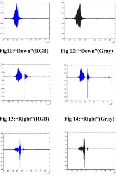
SIMULATION

Fig11:“Down”(RGB) Fig 12: “Down”(Gray)

Fig 13:“Right”(RGB) Fig 14:“Right”(Gray)

Fig 15

:“

Fig 5:“Aswini”(RGB) Fig 6:“Aswini”(Gray)

Fig 7: “Rahul”(RGB) Fig 8:“ Rahul”(Gray)

Fig 9: “Sunday”(RGB) Fig 10:“Sunday”(Gray)

Table 1.Comparison of Correlation Coefficients between the gray scale plot of sample word and stored words

word

Nilamadhab Soumya Aswini9 Rahul Sunday Up Down Left Right Status

Soumya 0.2194 0.3690 0.2365 0.2363 0.2118 0.3016 0.2926 0.3130 0.1494 match

Sunday 0.4360 0.4972 0.3597 0.3749 0.5715 0.4718 0.4972 0.3518 0.3760 match

Rahul 0.3212 0.3719 0.3241 0.5514 0.4122 0.2011 0.5763 0.3321 0.3146 mismatch

Up 0.2098 0.2234 0.2111 0.3211 0.3389 0.4355 0.2563 0.3243 0.3234 match

Aswini9 0.6224 0.7566 0.8925 0.6455 0.8322 0.6122 0.5567 0.7145 0.6201 match

Left 0.3215 0.3421 0.2451 0.3013 0.3112 0.2787 0.2345 0.4487 0.4782 mismatch

Nilamadhab 0.8755 0.6561 0.6324 0.7563 0.7312 0.6711 0.6656 0.6144 0.6367 match

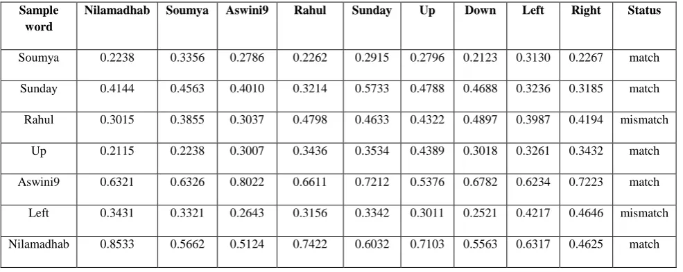
Table 2.Comparison of Correlation Coefficients between the histogram of sample word and stored words

word

Nilamadhab Soumya Aswini9 Rahul Sunday Up Down Left Right Status

Soumya 0.2238 0.3356 0.2786 0.2262 0.2915 0.2796 0.2123 0.3130 0.2267 match

Sunday 0.4144 0.4563 0.4010 0.3214 0.5733 0.4788 0.4688 0.3236 0.3185 match

Rahul 0.3015 0.3855 0.3037 0.4798 0.4633 0.4322 0.4897 0.3987 0.4194 mismatch

Up 0.2115 0.2238 0.3007 0.3436 0.3534 0.4389 0.3018 0.3261 0.3432 match

Aswini9 0.6321 0.6326 0.8022 0.6611 0.7212 0.5376 0.6782 0.6234 0.7223 match

Left 0.3431 0.3321 0.2643 0.3156 0.3342 0.3011 0.2521 0.4217 0.4646 mismatch

Nilamadhab 0.8533 0.5662 0.5124 0.7422 0.6032 0.7103 0.5563 0.6317 0.4625 match

6.

RESULTS AND DISCUSSIONS

The proposed algorithm prompts for inputting a specific word through the microphone. It matches the word with the words which are already stored in the database through the grayscale image and histogram plot. It performs the comparison by computing the co-relation coefficients and retrieves the word having maximum value of correlation coefficients. Generally we speak into a microphone connected to the computer and the soundcard or multimedia chip and the speech engine process the speech. The main problem is that speech is distorted by a background noise and echoes, electrical characteristics. Vocalizations may vary in terms of pronunciation, accent, articulation, and nasality, roughness in the voice while speaking, pitch, volume, and speed and therefore accuracy of speech wouldn’t be maintained. Along with it one should take care about the time duration while speaking in the microphone. The maximum delay should be within 1 to 2 sec. If more delay occurs then it may show the incorrect match. Detailed analysis of the algorithm tells that most of the time it is showing the match with the gray scale

7.

CONCLUSION AND FUTURE WORK

Speech recognition (by a machine) is a very complex problem. The performance of speech recognition systems is usually evaluated in terms of accuracy and speed. Speech is distorted by a background noise and echoes and therefore the physical shape of the graph changes to some extent. If this change is minimum, then the basic characteristics of the voice are not lost and correlation coefficient can find the exact match. But if the percentage of change is more, then the correlation coefficient may not show the exact match.Threfore we should be very much careful while inputting the sample voice Accuracy of speech recognition also vary with the vocabulary size and confusability, speaker dependence or independence, discontinuous, or continuous speech etc.The future work of this algorithm is to remove these external noise described above while inputting sample voice of sample word so that it will give the exact match. This algorithm is also showing the incorrect match for the words ending with same pronunciation. Therefore another solution is to train the system in such a way that the basic characteristics will not be lost even if in the noise distortion. This extra information represents characteristics of the talker such as emotional state, speech mannerisms, accent, etc., but much of it is due to the inefficiency of simply sampling and finely quantizing analog signals.

8.

REFERENCES

[1] Rabiner, L.R, Schafer, R.W. 2007. Introduction to Digital Speech Processing, Foundations and Trends_in Signal Processing Vol. 1, Nos. 1–2 (2007) 1–194.

[2] Tebllskis, J. 1995.Speech Recognition using Neural Network, Doctoral Thesis, Camegie Mellon University, Pittsburg, Pennsylvania.

[3] Lee, C.,Hyun, D.,Choi, E.,Go, J.,Lee, C. 2003.Optimizing feature Extraction From Speech Recognition.IEEE Transactions on Speech and Audio Processing Vol 11 No 1 P-80-86.

[4] Ohtsuki, K.,Matsunaga, S.,Matsuoka, T.,Furui, S. 1997.Topic Extraction Based on Continious Speech Recognition in Broadcast News Speech. . In Proceedings of the IEEE Conference on Automatic Speech Recognition and Understanding.

[5] Johnson, S. 2006. Stephen Johnson on Digital Photography. O'Reilly. ISBN- 0-596-52370-X.

[6] IDL. 2009 Image processing. Version 7.1.

[7] Kumar, T.,Verma, A.K. 2010.A Theory Based on RGB image to Gray Image,International Journal Of Computer Applications(0975-8887)Volume 7-No.2.

[8] Pratt, W.K. 1991.Digital Image Processing,Third Edition,John Wiley And Sons.

[9] Pearson, K. 1895. Contributions to the Mathematical Theory of Evolution. II. Skew Variation in Homogeneous Material. Philosophical Transactions of the Royal Society A: Mathematical, Physical and Engineering Sciences 186: 343–326.

[10]Hand, D.,Mannila, H.,Sannella, M.,Smyth, P. 2001.Principles of Data Mining, MIT Press, Massachusetts. J.