A FRAMEWORK FOR ARABIC SENTIMENT ANALYSIS USING MACHINE LEARNING CLASSIFIERS

4547

LOCALIZING MULTIPLE SCLEROSIS LESIONS FROM T2W

MRI BY UTILIZING IMAGE HISTOGRAM FEATURES

BAYDAA TAHA AL-HAMADANI

Computer Science Dept., Zarqa Universirt, Jordan. P.O.Box 132222, Zarqa, Jordan, 13132 Email: [email protected]

ABSTRACT

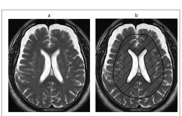
Multiple Sclerosis (MS) is one of the most frequent causes of permanent disability in young adults by damaging the central nervous system through the demyelinating process. As most of the demyelinating diseases, MS is asymptomatic. Hence, to diagnose and monitor the progress of MS patients, brain Magnetic Resonance Imaging (MRI) is used in order to localize MS lesions. According to McDonald’s criteria, white lesions, appeared in T2W MRIs, in callosum and periventricular areas are typical.

In this context, this paper proposed a fast localization and segmentation algorithms to localize MS lesions based on histogram features besides morphological features such as place, area, and intensity of the lesions appeared in the monitored places. The segmentation algorithm supplies the radiologist with the area of the detected lesions which considered to be valuable information in the process of monitoring the progress of the disease.

The evaluation procedures were carried out using two different clinical databases with 664 brain MR images. The results showed that the proposed technique achieved competitive sensitivity, specificity, predictive, and accuracy with 90.4, 95.6, 96.4, and 92.1 respectively. The average overall execution time with 12.3ms is considered to be fast compared with other proposals.

Keywords: Multiple Sclerosis, Histogram Equalization, Morphological Features, Magnetic Resonance Imaging, Texture Features, Localizing Lesions, Segmenting Lesions.

1. INTRODUCTION

Multiple Sclerosis (MS) is the most autoimmune demyelinating disease which causes serious damage to the central nervous system [1]. During the past few years, this disease increased dramatically causing serious symptoms such as optic neuritis and sensory problems, and it might cause permanent disability in patients with an average age of 29.2 years [2, 3].Thus, scientists in different fields such as clinical, physical and technological scientists are trying their effort in order to diagnose and control the disease, and monitor the patient’s treatment.

The progression of MS cannot be detected through particularly known symptoms or specific laboratory tests. For this reason, Magnetic Resonance Imaging (MRI) become the significant way, since 2001, in the process of managing patients with MS [4]. According to McDonald’s criteria for MS [5] and its revisions [6-8], the process of diagnosing MS cannot be done by clinical symptoms only, it should be accompanied by brain and spinal cord MR images where white

lesions appear in the Callosum, periventricular, and juxtacortical of the brain. These lesions are disseminated in time, where new lesions appeared, and space, where multiple lesions appeared. T2-weighted (T2W) MRI becomes a standard way of the diagnosing procedure since brain and spinal cord lesions appear clearly.

4548 Detecting and segmenting MS lesions manually by a physician is an effort, time and money consuming process. Moreover, it is not easy to segment MS lesions from between other lesions and matters and normal brain tissue. Thus there is a discernible need for automatic detection and segmenting MS lesions. This epidemiological disease attracts the attention of several researchers, and their researches were located into two main categories, which are either to understand the nature of the disease and how to diagnose and deal with it in one group and to detect and segment MS lesions in the another group automatically. Researches of the first group can be categorized being either to discuss MS nature, symptoms, ways of diagnosing, prevalence rate around the world, and treatment [2, 5, 11-15]; while other researches aimed to spot the light on the importance and techniques of using MRI in diagnosing and monitoring the progress of MS[4, 16-18]. Whilst in the second group, several techniques were proposed to localize and segment MS lesions beside several reviews that described and evaluated the performance of these techniques [19-23].These researches can be divided into two main categories, either supervised or unsupervised techniques.

Supervised techniques are supported by supervised algorithm such as spatially varying statistical classification (SVC), as in [24, 25], which employed a K-Nearest Neighbor (k-NN) classification scheme based on a template registration process to extract features from both normal MRI and MS patient MRI. While [26, 27]used multi-channel and context-rich random decision forest classifier by distinguishing the symmetric features of MS lesions and the mid-sagittal of the brain. In their works, [23] proposed OASIS to be an automated statistical method to estimate the presence of lesions depending on depending on voxel-level probabilities. Other methods depend on a variety of techniques such as [28] which depend on comparing images examples from Atlas to match patches using sparse dictionary; and [29, 30] that used multi-output decision trees to averaging multi-layers images; [31] which deployed SVM with longitudinal lesion segmentation.

On the other side, most proposed techniques were unsupervised that based on statistical and morphological features to outline MS lesions. One of the early proposed methods were [32] who depend on the tissue intensity distribution parameters to distinguish between MS lesions and normal brain tissue. In 2003, [33, 34] utilized a support vector machine (SVM)classifier in order to normalize tissue intensities. Later, [35]used multi-sequence segmentation and Trimmed

a  b 

4549 Likelihood Estimator (TLE) to outline MS lesions depending on the prior information. The same technique had been improved later by, by [36] in the way of combining it with a Hidden Markov Chain (HMC),and further improvement had been done later by [37, 38] in the way of combining it with Mean Shift to exclude the regions which are outliers. Later [39] proposed a new segmentation approach based on the morphological features extracted by using the gray-level co-occurrence matrix (GLCM) and the gray-level run length matrix (GLRLM).

In this paper, we propose a new localization and segmentation approach based on comparing the MS patient’s MRI with a template image for a healthy person to highlight outlier area after extracting specific texture and morphological features to distinguish these areas from normal brain tissue based on the histogram equalization technique.

2. MATERIAL

Two MRI datasets were used in the evaluation phase of the proposed technique. These datasets were varying to cover all four

types of MS which are secondary progressive, primary progressive,relapsing-remitting, and isolated clinical syndrome. The detailed description of the dataset are listed in the following subsections:

a.eHealth Laboratory dataset[40-43]: which is published for free by the Department of Computer Science in the University of Cyprus. It contains 38 T2W MRI obtained by a turbo spin echo pulse sequence with echo spacing of 10.8 ms, echo timing of 100 ms, and repetition timing of 4408 ms.

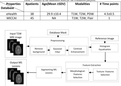
b.MICCAI[44]: which is published for free by the Neuroimaging Informatics Tools and Resources Clearinghouse (NITRC) and the MRIs were gathered at the University of North Carolina and Children’s Hospital Boston. It contains 45 T2W MRI with0.5 as slices thickness. The T2 weighted images were registered to its corresponding T1,which are already registered to the standard MNI Atlas format [45]. More details about the used databases are listed in Table 1.

Table 1: Details of the databases used for the evaluation purpose.

       Properties  Database 

#patients  Age(Mean ±SDV)  Modalities  # Time points 

eHealth  38  29.9 ±10.4  T1W, T2W, PDW  4.5±0.5 

MICCAI  45  NA  T1W, T2W, Flair  1 

Input T2W  MRI image 

Database Mask

Remove  background 

Gaussian  Filter 

Contrast  Enhancement  Preprocessing

  Morphological‐ Features  Selection 

Texture‐ Features  Selection  Feature Extraction 

Reference Image 

Histogram  Equalization 

Segmenting MS  Lesions 

Output MS  Lesions 

4550

3. METHODOLOGY

The main purpose of MS Lesions Localization (MSLL) is to localize MS lesions that are located in Callosum and Periventricular areas in the brain. According to McDonalds criteria, besides spinal cord lesions, white lesions in these two areas are compulsory to diagnose MS, while other white matters that appeared in other parts could be caused by other diseases rather than MS [46]. The proposed technique has the ability to assist physicians in improving the process of interpreting medical images to be more accurate, fast, and efficient. Besides, MSLL supply the physician with useful information, such as the location, number, and size of the lesion(s) to be used for comparing MR images. As illustrated in Figure 2, the proposed MSLL consists of several stages: preprocessing,

histogram equalization, feature extraction, and segmentation.

3.1 Preprocessing

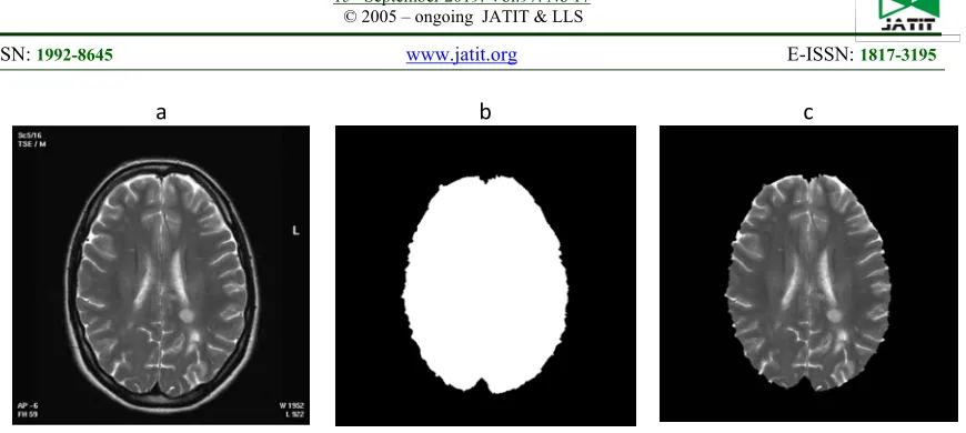
The input to this stage is an MR T2W image and an image mask which is generated automatically for each database. The dimensions and formats of each used databases are different due to the differences in the scanner devices used, this reason behind using an image mask as another input for the preprocessing stage. As shown in Figure 3 (a), the MR images contain distracting background details which can affect the results of MSLL since it depends on the differences in the image histogram of a healthy person and a patient with lesions.

a  b  c 

Figure 3: Steps Of Removing Unwanted Background.

a  b  c 

4551 As in Eq.(1), removing unwanted background is done by multiplying the MR original image (Figure 3 (a)) by the generated mask (Figure 3 (b)) to produce the new MRI (Figure 3 (c)).

𝑄 𝑖, 𝑗 𝑀𝑅𝐼 𝑖, 𝑗 𝑀 𝑖, 𝑗 ……….. (1)

As a second step of the preprocessing stage, a 3X3 Gaussian filter is applied to reduce false positive ratio, minimize noise effects, and smooth the image. In Eq. (2), f1(x, y) is the Gaussian filter which applied onto 𝑄 𝑖, 𝑗 , where 𝜎 represents the standard variation.

𝑓1 𝑥, 𝑦 𝑒 ……….(2)

The resultant image is shown in Figure 4 (b), and the applied filter is visualized in Figure 4 (a) with 𝜎 0.7. The result of applying Gaussian filter makes the required details become blur. To enhance the image and increase the contrast between bathe ckground and other matters in the image, Eq. (3) is applied and the resultant image is shown in Figure 4 (c). T1 and T2 are two

selected threshold values which are chosen to highlight the required lesions.

𝑄 𝑖, 𝑗 1 𝑖𝑓 𝑇 𝑄 𝑖, 𝑗 𝑇

𝑄 𝑖, 𝑗 , 𝑜𝑡ℎ𝑒𝑟𝑤𝑖𝑠𝑒   ……… 

(3) 

3.2 Histogram Equalization

The process of histogram equalization had been used in several previous types of research in order to reduce the differences between images

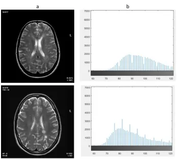
that were taken using different scanners [47-50]. This method can reduce the variation in white matter intensities (MS lesion in our case) from 7.5

a  b 

4552 to 2.5%. Furthermore, the histogram of a healthy

a  b  c 

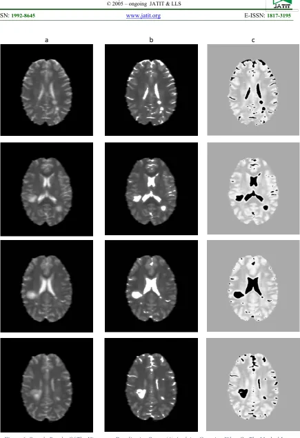
4553 MRI has big differences than this with white lesions. Figure 5 illustrates an example of two MRIs alongside with their histogram, a healthy image (top row) and an image with MS (bottom row).For all the aforementioned reasons, MSLL

depends on histogram equalization of a healthy image (reference image) with the input image in order to increase the intensities of MS lesions comparing to other normal brain tissue. Four contrast enhancement (column (b)), and then equalizing its histogram with the required dataset reference image (column (c)).sample images were after applying Gaussian filter on the masked image (column (a)), chosen for the purpose of explaining the results of each stage.

Figure 6 shows the resultant images

3.3 Features Extraction

The results of the histogram equalization stage are converted into black and white images according to a specific threshold in order to spot the light on several candidate regions, most of them are false positives. Feature extraction stage reduces these regions and identifies each region by either MS lesion or normal brain tissue. Two types of features are used, first-order features and second-order features. In first-order features, the texture of the candidates is selected, while, on the other hand, morphological features are selected in the second-order.

3.3.1 Texture-Features Selection

The purpose of this stage is to reduce the number of candidates based on specific features corresponding to the histogram intensity level of MS lesions. These features are intensity mean, standard deviation, and smoothness (Table 2). In this stage, some lesions rather than MS are excluded, since MS lesions appear in MRIs as

light-gray to white lesions with almost constant intensity level, while, for instance, cavernoma disease produces popcorn shape lesions that have completely different values of 𝜇, 𝜎, 𝑎𝑛𝑑 𝜑.

Table 2: Texture features used in MSLL.

Where, Rw and Rh are the width and height of the candidate region R, respectively, and Λ represents the number of pixels in R.

3.3.2 Morphological Features Selection

Morphological features can be divided in our proposed work into two parts, either mathematical morphology or location morphology. Mathematical morphology is a way used for extracting specific features from the candidate regions such as shape and size [51, 52]. Most MS lesions tend to be circular to oval shape lesions but they can be irregular [53], but after applying morphological functions (dilation in Eq. (4) and erosion in Eq. (5)), these irregular lesions turned to be close to a circular shape.

𝛿𝑓 𝑥, 𝑦 max 𝑓 𝑥 𝑠, 𝑦 𝑡

𝑏 𝑠, 𝑡 | 𝑥 𝑠, 𝑦 𝑡 ∈ 𝐷 ; 𝑠, 𝑡 ∈ 𝐷

………. (4)

𝜀𝑓 𝑥, 𝑦 min 𝑓 𝑥 𝑠, 𝑦 𝑡

𝑏 𝑠, 𝑡 | 𝑥 𝑠, 𝑦 𝑡 ∈ 𝐷 ; 𝑠, 𝑡 ∈ 𝐷

……... (5)

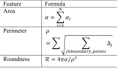
On the other hand, other morphological features can be used to reduce the number of false positive candidates such as location, area, and circular roundness value. The applied features are listed in Table 3. The detailed procedure of applying these features is illustrated in Algorithm-1.

Table 3: Morphological features used in MSLL.

Feature Formula

Area

𝛼 𝛼

Perimeter 𝜌

∆

∈ _

Roundness ℛ 4𝜋𝛼/𝜌

Feature Formula

Intensity

mean _𝜇 1

𝑅 ∙ 𝑅 𝑅 𝑖, 𝑗

Standard deviation 𝜎

1

Λ 1 𝑅 𝑖, 𝑗 𝜇

Smoothness

𝜑 1 1

4554

After specifying whether a selected candidate’s center lies inside the periventricular and corpus callosum region, the roundness feature can be used to specify whether it is an MS lesion or not with a threshold of 0.75.All candidates that are outside the required MS region or have ℛ

Algorithm-1: Applying_Morphological_Features(A, R, n) Input: a List of all candidate regions (A) of length n

MS region of interest (R) which illustrated in Figure 1(b)

Output: a list of MS lesions

∀𝑎 | 𝑎 ∈ 𝐴, 𝑖 𝑛

𝒊𝒇𝑎, ⊚ 𝑅 // if the selected candidate center (i,j) lies inside R

Create ℬ 𝑥, 𝑦 : a list of all boundary-points coordination Create ℬ 𝑥, 𝑦

for n=1to ℬ.size-1

for m=1to ℬ.size-1

ℬ 𝑛, 𝑚 ℬ 𝑛 1, 𝑚 1 ℬ 𝑛, 𝑚

𝑎 ℬ 𝑥, 𝑦

𝑎 𝑎,. 𝑎𝑟𝑒𝑎

𝑎ℛ 4𝜋𝑎 /𝑎

𝒊𝒇𝑎ℛ 0.75

4555

𝑇ℎ𝑟𝑒𝑠ℎ𝑜𝑙𝑑 are discarded. Figure 7 illustrates

examples of implementing MSLL where column

(a) represents the B/W images of the histogram equalization stage.

a  b  c  d 

Figure 7: results of Morphological features, (a) converting the histogram Equalization stage results into B/W, (b) candidate regions with  the roundness value, (c) results of texture features selection to remove part of the false positive candidates, and (d) morphological 

4556 The candidate regions are colored and the roundness values are written in column (b) and then the results of texture features selection are in column (c). Finally, the results of removing all the remaining false positive candidates using morphological features are illustrated in column (d).

3.4 Segmentation

The last step in localizing MS lesions is to localize the whole lesion by adopting the

algorithm used in [54] to localize a whole Optic disk from a fundus image. The algorithm starts from the horizontal radius line and tries to expand it on both sides base on the intensity level of each pixel and then the same process returns to be done on the vertical radius line. Figure 8 shows an example of an MS lesion in (a). The result of all the pre-mentioned stages is shown in (b), and the result of the segmentation algorithm is in (c).

Algorithm-2: Localizing_Whole_MSLesion (A, n) Input: a List of all MS lesions (A) of length n Output: a list of whole MS lesions

∀𝑎 | 𝑎 ∈ 𝐴, 𝑖 𝑛

Let (a,b) be the center of 𝑎

Let𝑐 be the circle surrounding 𝑎 with radius r and passing through a point 𝑥, 𝑦 , such that:𝑟 𝑥 𝑎 𝑦 𝑏 while true // Expand 𝑐 .radius horizontally from the right side

Let𝑘 𝑥́, 𝑦́ be a point outside 𝑐 and 𝑟 𝑥, 𝑦 be a point on the intersection of 𝑟 𝑎𝑛𝑑 𝑐 | 𝑥́ 𝑥, 𝑎𝑛𝑑 𝑦́ 𝑦 1

if𝑘 𝑥́, 𝑦́ 𝐼𝑛𝑡𝑒𝑛𝑠𝑖𝑡𝑦 𝑟 𝑥, 𝑦 𝑟 𝑥, 𝑦́

else return false

while true // Expand 𝑐 .radius horizontally from the left side

Let𝑘 𝑥́, 𝑦́ be a point outside 𝑐 and 𝑟 𝑥, 𝑦 be a point on the intersection of 𝑟 𝑎𝑛𝑑 𝑐 | 𝑥́ 𝑥, 𝑎𝑛𝑑 𝑦́ 𝑦 1

if𝑘 𝑥́, 𝑦́ 𝐼𝑛𝑡𝑒𝑛𝑠𝑖𝑡𝑦 𝑟 𝑥, 𝑦 𝑟 𝑥, 𝑦́ else return false

while true // Expand 𝑐 .radius vertically from the top side

Let𝑘 𝑥́, 𝑦́ be a point outside 𝑐 and 𝑟 𝑥, 𝑦 be a point on the intersection of 𝑟 𝑎𝑛𝑑 𝑐 | 𝑥́ 𝑥 1, 𝑎𝑛𝑑 𝑦́ 𝑦

if 𝑘 𝑥́, 𝑦́ 𝐼𝑛𝑡𝑒𝑛𝑠𝑖𝑡𝑦 𝑟 𝑥, 𝑦 𝑟 𝑥́, 𝑦

else return false

while true // Expand 𝑐 .radius vertically from the bottom side

Let𝑘 𝑥́, 𝑦́ be a point outside 𝑐 and 𝑟 𝑥, 𝑦 be a point on the intersection of 𝑟 𝑎𝑛𝑑 𝑐 | 𝑥́ 𝑥 1, 𝑎𝑛𝑑 𝑦́ 𝑦

if𝑘 𝑥́, 𝑦́ 𝐼𝑛𝑡𝑒𝑛𝑠𝑖𝑡𝑦 𝑟 𝑥, 𝑦 𝑟 𝑥́, 𝑦

else return false

4557

4. EVALUATION AND COMPARISONS

This section discusses the quality of MSLL first by evaluating its performance in terms of specific factors and second by comparing its overall performance and evaluation time with competitive proposals.

4.1 Evaluation

The evaluation of MSLL is done by measuring specific factors which are accuracy percent, sensitivity, specificity, and computational time. Firstly, the accuracy percent is calculated to emphasize the performance of MSLL in localizing and segmenting MS lesions accurately using Eq. (6).

𝐴𝑐𝑐 𝑥 100 ………..

(6)

Accuracy percent, (Acc) for a specific database (𝑥) with 𝑁 images, is the number of images in which the specific algorithm was successfully implemented and achieved its goal (𝑥 ) divided by (𝑁). The results of this factor in localizing and segmenting MS lesions are listed in Table 4 and Table 5 respectively.

Table 4: Accuracy percent of MSLL localizing MS  lesions and the overall accuracy average. 

      Database  Property      

eHealth  MICCAI 

#images  304  360  #success  267  346  Acc  87.88  96.11 

Average Acc  91.99   

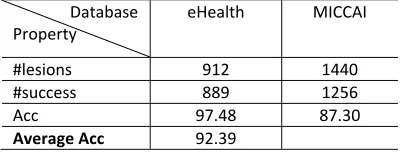
Table 5: Accuracy percent of MSLL segmentation  whole MS lesions the overall accuracy average. 

      Database  Property      

eHealth  MICCAI 

#lesions  912  1440  #success  889  1256  Acc  97.48  87.30 

Average Acc  92.39   

As noticed from the accuracy average results, the designed MSLL achieved significant results in both localizing and segmented MS lesions. Figure 10 contains sample results from both of the used databases (eHealth and MICCAI), in which the first and third columns are the original MRIs, while the second and the fourth are the results of implementing MSLL. As seen in the figure, MS lesions are surrounded by a circle, and the approximate area of each lesion is indicated beside it. This piece of information about the area of the MS lesion is very important in the process of monitoring the patient’s case by comparing his/her MRIs every six months to evaluate if there is any dissemination in space and/or time based on Mc Donald’s criteria.

Nevertheless, MSLL fails in localizing some or all of the lesions for several reasons. Figure 9 shows examples of failed MSLL implementation where the red circles are made by a radiologist. In the first three images (a, b, and c) the intensity level of unlocalized MS lesions are close to the background’s expert while the last example image (d) has a different angle than other images which makes the mask image fails to detect the background.

a  b  c 

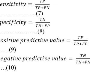
4558 As a second step in the evaluation process, the sensitivity, specificity, and positive and negative predictive values, which are indicated in Eq. (7), (8), (9), and (10) respectively, were used. To reach this goal, a radiologist marked the MS lesions in the tested images and their results were compared to what has been achieved by MSLL in both sides, the MS localization and MS segmentation.

𝑠𝑒𝑛𝑠𝑖𝑡𝑖𝑣𝑖𝑡𝑦

………..(7)

𝑠𝑝𝑒𝑐𝑖𝑓𝑖𝑐𝑖𝑡𝑦

…...………(8)

𝑝𝑜𝑠𝑖𝑡𝑖𝑣𝑒 𝑝𝑟𝑒𝑑𝑖𝑐𝑡𝑖𝑣𝑒 𝑣𝑎𝑙𝑢𝑒

……(9)

𝑛𝑒𝑔𝑎𝑡𝑖𝑣𝑒 𝑝𝑟𝑒𝑑𝑖𝑐𝑡𝑖𝑣𝑒 𝑣𝑎𝑙𝑢𝑒

.….(10)

In the side of evaluating the localization procedure, true positive (TP) represents the

number of MS lesions correctly detected, false positive (FP) is those which are detected wrongly as MS lesions, false negative (FN) is the number of MS lesions that were not detected, and true negative (TN) is the number of non-MS lesions which were correctly identified as non-MS lesions. Table 6 lists the results of these evaluation factors for selected image samples.

4559

Original  Result  Original Result

Figure 10: Sample results of MSLL where the first and third columns are original MRIs, while the seconf and fourth columns are the results of MSLL.

a  b c d

4560

Table 6: Evaluation Of MSLL Localization Procedure In Terms Of Sensitivity, Specificity, And Positive And Negative Predictive Factors.

Image number

TP FP TN FN Sensitivity

% Specificity % +Predictive % -Predictive % Time/ms

IMR1 3 1 7 1 75.00 87.50 75.00 87.50 12

IMR2 3 0 6 1 75.00 100.00 100.00 85.71 12.5

IMR3 4 1 6 1 80.00 85.71 80.00 85.71 12.7

IMR4 4 0 5 1 80.00 100.00 100.00 83.33 13.1

IMR5 4 0 6 1 80.00 100.00 100.00 85.71 13.0

IMR6 5 1 6 2 71.43 85.71 83.33 75.00 12.9

IMR7 2 1 9 0 100.00 90.00 66.67 100.00 11.8

IMR8 1 2 5 1 50.00 71.43 33.33 83.33 10.9

IMR9 3 1 6 1 75.00 85.71 75.00 85.71 11.9

IMR10 4 0 5 1 80.00 100.00 100.00 83.33 12.3

IMR11 3 1 4 0 100.00 80.00 75.00 100.00 12.6

IMR12 3 0 5 1 75.00 100.00 100.00 83.33 11.8

IMR13 4 1 4 1 80.00 80.00 80.00 80.00 13.0

IMR14 4 0 3 0 100.00 100.00 100.00 100.00 13.4

IMR15 5 0 8 0 100.00 100.00 100.00 100.00 13.6

Average 90.43 93.07 87.56 90.91 12.9

As noticed from the measured factors, MSLL accomplish a high sensitivity in both localization and segmentation algorithms, which show that high numbers of MS lesions are localized correctly with the maximum amount of their pixels were segmented. Moreover, more than 60% of the tested images have their FN value equals to 0 which means that the technique localizes most of the MS lesions. The average specificity, on the other hand, is considered to be high which indicates that the proposed technique has good ability to exclude none MS lesions from the

resultant segmented regions. The values of positive and negative predictive are used to measure the accuracy of our technique. The average values of these measurements show that MSLL has high accuracy since it has a high priority of detecting MS lesions as MS lesions (positive prediction) and none-MS lesions as non-MS lesions(negative prediction). On the other hand, the average time required for both the localization and segmentation algorithms using Intel Core-i7 CPU with 2.7GHz speed is 12.3ms which considered being fast.

Table 7: Evaluation Of MSLL Segmentation Procedure In Terms Of Sensitivity, Specificity, And Positive And Negative Predictive Factors.

Image number

TP FP TN FN Sensitivity %

Specificity %

+Predictive %

-Predictive

%

Time/ms

IMR1 2729 0 259415 110 96.13 99.96 96.13 99.96 11.1

IMR2 387 12 261757 18 95.56 99.99 95.56 99.99 12.3

IMR3 563 5 261581 87 86.62 99.97 86.62 99.97 11.2

IMR4 1721 14 260423 76 95.77 99.97 95.77 99.97 10.3

IMR5 659 0 261485 34 95.09 99.99 95.09 99.99 9.8

IMR6 876 4 261268 97 90.03 99.96 90.03 99.96 10.4

IMR7 283 22 261861 33 89.56 99.99 89.56 99.99 15.5

IMR8 76 3 262068 12 86.36 100.00 86.36 100.00 9.9

IMR9 127 12 262017 25 83.55 99.99 83.55 99.99 13.4

IMR10 324 0 261820 117 73.47 99.96 73.47 99.96 8.6

IMR11 1270 7 260874 155 89.12 99.94 89.12 99.94 11.7

IMR12 763 10 261381 133 85.16 99.95 85.16 99.95 13.8

IMR13 734 0 261410 58 92.68 99.98 92.68 99.98 7.3

IMR14 1376 0 260768 332 80.56 99.87 80.56 99.87 8.3

IMR15 877 9 261267 52 94.40 99.98 94.40 99.98 11.6

4561

4.2 Comparisons

This section discusses the results of comparing the final results of our proposed MSLL with other state-of-the-art proposals. Table 8 compares the performance of MSLL against five other proposals in terms of sensitivity, specificity, predictive, and accuracy. The results show that MSLL has competitive values of the selected factors, although some of the proposed techniques are exceeding MSLL since most of these proposals used some learning machine algorithms which increase their performance.

Table 8: Comparing MSLL with some of the state-of-the-art techniques.

Author Sensitivit

y % Specificit y % Predictiv e % Accurac y % Nayak

D. R. et al. [22]

96.01 96.70 95.72 96.40

Ghribi

O. et

al.[39]

76 78 - 73

Bauer S. et al.[25]

83 79 - 80

Murray V. et al. [23]

94.08 93.64 91.91 93.83

Zhang Y. et al. [55]

96.15 97.16 96.30 96.72

The propose d MSLL

90.4 95.6 96.4 92.1

5. CONCLUSION AND FUTURE

SUGGESTIONS

MS is considered as one of the most disabling diseases especially among young people. Several computer-based techniques were proposed in order to detect and monitor the progress of MS based on MR images. This paper proposed a fully automated technique that uses the histogram equalization algorithm and morphological features to localize MS lesions in both Callosum and Periventricular areas in the brain. After detecting the lesions, the process of segmenting them starts to calculate the approximate area of these lesions in order to help specialists in the process of monitoring the patient’s case in both space and time dissemination. The performance of the proposed technique is considered to be competitive

comparing to other proposals by achieving 90.4, 95.6, 96.4, and 92.1 for sensitivity, specificity, predictive, and accuracy respectively. The required average executions time is 12.3ms which considered being fast.

Some improvements are needed to increase MSLL performance by using a learning machine algorithm such as support vector machine (SVM) to select the required features from the image and use them to decide whether a specific lesion is an MS or not.

ACKNOWLEDGMENT

This research is funded by the Deanship of Scientific Research in Zarqa University /Jordan.

REFERENCES

[1] Organization, W.H., Atlas: Multiple Sclerosis Resources in the World 2008, G. Springer, Switzerland, Editor 2008.

[2] Leray, E., et al., Epidemiology of multiple sclerosis. Revue Neurologique, 2016. 172(1): p. 3-13.

[3] Dahan, A., W. Wang, and F. Gaillard,

Computer-Aided Detection Can Bridge the Skill Gap in Multiple Sclerosis Monitoring.

Journal of the American College of Radiology, 2018. 15(1, Part A): p. 93-96. [4] Wattjes, M.P., M.D. Steenwijk, and M.

Stangel, MRI in the Diagnosis and Monitoring of Multiple Sclerosis: An Update. Clinical Neuroradiology, 2015. 25(2): p. 157-165.

[5] McDonald, W.I., et al., Recommended Diagnostic Criteria for Multiple Sclerosis: Guidelines from the International Panel on the Diagnosis of Multiple Sclerosis. Ann Neurol 2001. 50(1): p. 121-127.

[6] AJ, T., et al., Diagnosis of multiple sclerosis: 2017 revisions of the McDonald criteria.

Lancet Neuro, 2018. 17(2): p. 162-173. [7] Polman, C.H., et al., Diagnostic criteria for

multiple sclerosis: 2005 revisions to the “McDonald Criteria”. Ann Neurol, 2005. 58(1): p. 840-46.

[8] Polman, C.H., et al., Diagnostic criteria for multiple sclerosis: 2010 revisions to the McDonald criteria. Ann. Neurol, 2011. 69: p. 292-302.

4562 from:

http://www.pediatrics.emory.edu/divisions/ neonatology/dpc/pvhivh.html.

[10] Pekala, J.S., et al., Focal Lesion in the Splenium of the Corpus Callosum on FLAIR MR Images: A Common Finding with Aging and after Brain Radiation Therapy.

American Journal of Neuroradiology, 2003. 24(1): p. 855-861.

[11] Thouvenot, E., Multiple sclerosis biomarkers: Helping the diagnosis? Revue Neurologique, 2018.

[12] Waldman, A.T., et al., Binocular low-contrast letter acuity and the symbol digit modalities test improve the ability of the Multiple Sclerosis Functional Composite to predict disease in pediatric multiple sclerosis. Multiple Sclerosis and Related Disorders, 2016. 10: p. 73-78.

[13] Popescu, V., et al., Grey Matter Atrophy in Multiple Sclerosis: Clinical Interpretation Depends on Choice of Analysis Method.

PLoS ONE, 2016. 11(1).

[14] Lundmark, F., et al., Variation in interleukin 7 receptor α chain (IL7R) influences risk of multiple sclerosis. Nature Genetics, 2007. 39(2007): p. 1108-1114.

[15] Pugliatti, M., et al., The epidemiology of multiple sclerosis in Europe. European Journal of Neurology, 2006. 13(2006): p. 700-722.

[16] Louapre, C., Conventional and advanced MRI in multiple sclerosis. Revue Neurologique, 2018.

[17] Moccia, M. and O. Ciccarelli, Molecular and Metabolic Imaging in Multiple Sclerosis. Neuroimaging Clinics of North America, 2017. 27(2): p. 343-356.

[18] Horsfield, M.A., MR Image Postprocessing for Multiple Sclerosis Research.

Neuroimaging Clinics of North America, 2008. 18(4): p. 637-649.

[19] García-Lorenzo, D., et al., Review of Automatic Segmentation Methods of Multiple Sclerosis white Matter Lesions on Conventional Magnetic Resonance Imaging. Medical Image Analysis, 2013. 17(1): p. 1-18.

[20] Lladó, X., et al., Segmentation of multiple sclerosis lesions in brain MRI: A review of automated approaches. Information Sciences, 2012. 186(1): p. 164-185.

[21] Ghribi, O., et al. Brief review of multiplesclerosis lesions segmentation methods on conventional magnetic

resonanceimaging. in Proceedings of 1st Conference on Advanced Technologies for Signaland Image Processing (ATSIP 2014). 2014.

[22] Nayak, D.R., R. Dash, and B. Majhi, Brain MR image classification using two-dimensional discrete wavelet transform and AdaBoost with random forests.

Neurocomputing, 2016. 177(1): p. 188-197. [23] Murray, V., P. Rodríguez, and M.S. Pattichis, Multiscale AM-FM demodulation and image reconstruction methods with improved accuracy. IEEE Transactions on Image Processing, 2010. 19(1): p. 1138-1152.

[24] Warfield, S.K., et al., Adaptive, template moderated, spatially varying statistical classification. Medical Image Analysis, 2000. 4(1): p. 43-55.

[25] Bauer, S., L.-P. Nolte, and M. Reyes. Fully Automatic Segmentation of Brain Tumor Images Using Support Vector Machine Classification in Combination with Hierarchical Conditional Random Field Regularization. 2011. Berlin, Heidelberg: Springer Berlin Heidelberg.

[26] Geremia, E., et al. Spatial decision forests for MS lesion segmentation in multi-channel MR images. in 13th International Conference on Medical Image Computing and Computer Assisted Intervention (MICCAI 2010). 2010.

[27] Geremia, E., et al., Spatial decision forests for MS lesion segmentation in multi-channel magnetic resonance images. NeuroImage, 2011. 57(2): p. 378-390.

[28] Roy, S., et al., Example Based Lesion Segmentation, in Proceedings of SPIE Medical Imaging (SPIE-MI 2014)2014: San Diego, CA. p. 9034-90341.

[29] Amod Jog, et al. Multi-output decision trees for lesion segmentation in multiple sclerosis. in SPIE Medical Imaging (SPIEMI2015). 2015. Orlando, FL.

[30] WIDYANTARA, I.M.O., et al.,

AUTOMATED SHORELINE DETECTION DERIVED FROM VIDEO IMAGERY USING MULTI THRESHOLDING TECHNIQUES. Journal of Theoretical and Applied Information Technology, 2019. 97(5): p. 1500-1511.

4563 [32] Leemput, K.V., et al., Automated

segmentation of multiple sclerosis lesions by model outlier detection. IEEE Transactions on Medical Imaging, 2001. 20(8): p. 677 - 688.

[33] Ferrari, R.J., et al. Segmentation of multiple sclerosis lesions using support vector machines. in SPIE Medical Imaging (SPIE-MI 2003). 2003.

[34] CANDRADEWI, I., B.N. PRASTOWO,

and D. LATHIEF, GENDER

CLASSIFICATION FROM FACIAL IMAGES USING SUPPORT VECTOR MACHINE. journal of Theoretical and Applied Information Technology, 2019. 97(10): p. 2684-2692.

[35] A¨ıt-Ali, L.S., et al. STREM: a robust multidimensional parametric method to segment MS lesions in MRI. in 8th International Conference on Medical Image Computing and Computer Assisted Intervention (MICCAI 2005). 2005.

[36] Bricq, S., C. Collet, and J.-P. Armspach.

Lesion detection in 3D brain MRI using trimmed likelihood estimator and probabilistic atlas. in 5th International Symposium on Biomedical Imaging (ISBI 2008). 2008.

[37] Garcia-Lorenzo, D., et al., Trimmed-Likelihood Estimation for Focal Lesions and Tissue Segmentation in Multisequence MRI for Multiple Sclerosis. IEEE Transactions on Medical Imaging, 2011. 30(8): p. 1455 - 1467.

[38] García-Lorenzo, D., et al. Combining robust expectation maximization and mean shift algorithms for multiple sclerosis brain segmentation. in Workshop on Medical Image Analysis on Multiple Sclerosis (MIAMS2008). 2008. New York, United States.

[39] Ghribi, O., et al., Multiple sclerosis exploration based on automatic MRI modalities segmentation approach with advanced volumetric evaluations for essential feature extraction. Biomedical Signal Processing and Control, 2018. 40: p. 473-487.

[40] Loizou, C.P., et al., Multiscale Amplitude-Modulation Frequency-Amplitude-Modulation (AM– FM) Texture Analysis of Multiple Sclerosis in Brain MRI Images. IEEE Transactions on Information Technology in Biomedicine, 2011. 15(1): p. 119-129.

[41] Loizou, C.P., et al. Brain White Matter Lesions Classification in Multiple Sclerosis Subjects for the Prognosis of Future Disability. in Artificial Intelligence Applications and Innovations. 2011. Berlin, Heidelberg: Springer Berlin Heidelberg. [42] Loizou, C.P., et al. Brain MR image

normalization in texture analysis of multiple sclerosis. in 2009 9th International Conference on Information Technology and Applications in Biomedicine. 2009.

[43] Loizou, C.P., et al. Quantitative analysis of brain white matter lesions in multiple sclerosis subjects: Preliminary findings. in

2008 International Conference on Information Technology and Applications in Biomedicine. 2008.

[44] Clearinghouse, N.I.T.a.R. MICCAI 2008 Challenge website. 2008 [cited 2018 1-8-];

Available from:

http://www.ia.unc.edu/MSseg/results. [45] Styner, M., et al., 3D Segmentation in the

Clinic: A Grand Challenge II: MS lesion segmentation, in MIDAS Journal - MS Lesion Segmentation (MICCAI 2008 Workshop).2008.

[46] Barkhof, F., R. Smithuis, and M. Hazewinkel. Multiple Sclerosis. Radiology Assistant 2013 [cited 2018 12-8]; Available from:

http://www.radiologyassistant.nl/en/p4556

dea65db62/multiple-sclerosis.html#i459959844a779.

[47] Sun, X., et al., Histogram-based normalization technique on human brain magnetic resonance images from different acquisitions. BioMedical Engineering OnLine, 2015. 14(1): p. 73.

[48] Collewet, G., M. Strzelecki, and F. Mariette,

Influence of MRI acquisition protocols and image intensity normalization methods on texture classification. Magnetic Resonance Imaging, 2004. 22(1): p. 81-91.

[49] Meier, D.S. and C.R.G. Guttmann, Time-series analysis of MRI intensity patterns in multiple sclerosis. NeuroImage, 2003. 20(2): p. 1193-1209.

[50] Shah, M., et al., Evaluating intensity normalization on MRIs of human brain with multiple sclerosis. Medical Image Analysis, 2011. 15(2): p. 267-282.

4564 Journal of Clinical Bioinformatics, 2011. 1: p. 33-33.

[52] Serra, J., Image Analysis and Mathematical Morphology. 1983: Academic Press, Inc. [53] Sahraian, M.A. and E.-W. Radue, MS

Lesions in T2-Weighted Images, in MRI Atlas of MS Lesions, E.-W. Radü and M.A. Sahraian, Editors. 2008, Springer Berlin Heidelberg: Berlin, Heidelberg. p. 3-34. [54] Al-Hamadani, B.T., A fast template-based

technique to extract optic disc from coloured fundus images based on histogram features. International Journal of Signal and Imaging Systems Engineering 2018. 11(2): p. 117-127.

[55] Zhang, Y.-D., et al., Pathological brain detection in magnetic resonance imaging scanning by wavelet entropy and hybridization of biogeography-based optimization and particle swarm optimization. Progress In Electromagnetics Research, 2015. 152(1): p. 41-58.