Dynamic sensitivity analysis in Levy process driven option models

London School of Economics and Political Science Department of Statistics

D ynam ic S en sitivity A nalysis

in Levy P rocess D riven O ption

M odels

by

Adrian Urs Gfeller

London, March 2008

Supervisor Prof. Ragnar Norberg

UMI Number: U 615524

All rights reserved

INFORMATION TO ALL U SE R S

The quality of this reproduction is d ep en d en t upon the quality of the copy subm itted.

In the unlikely even t that the author did not sen d a com plete m anuscript

and there are m issing p a g e s, th e se will be noted. Also, if material had to be rem oved,

a note will indicate the deletion.

Dissertation Publishing

UMI U 615524

Published by ProQ uest LLC 2014. Copyright in the Dissertation held by the Author.

Microform Edition © ProQ uest LLC.

All rights reserved. This work is protected against unauthorized copying under Title 17, United S ta tes C ode.

ProQ uest LLC

789 East E isenhow er Parkway

tZQViV

■cjuaios J'uiouoO^pue

eoniKJ n toA jBXiiqWMe

A j B j q n

I certify that the thesis I have presented for examination for the PhD degree of the London School of Economics and Political Science is solely my own work other than where I have clearly indicated that it is the work of others. The copyright of this thesis rests with the author. Quotation from it is per­ mitted, provided that full acknowledgement is made. This thesis may not be reproduced without the prior written consent of the author.

I warrant that this authorisation does not, to the best of my belief, infringe the rights of any third party.

A cknow ledgem ents

I would like to express my gratitude to my supervisor Professor Ragnar Nor- berg for his guidance and support throughout my doctorate. His advice and help have been invaluable.

My thanks also go to the present and former members of the Statistics Department of the London School of Economics, both faculty and fellow students, for the stimulating discussions and for the delightful working at­ mosphere.

A bstract

Option prices in the Black-Scholes model can usually be expressed as so­ lutions of partial differential equations (PDE). In general exponential Levy models an additional integral term has to be added and the prices can be expressed as solutions of partial integro-differential equations (PIDE). The sensitivity of a price function to changes in its arguments is given by its derivatives, in finance known as greeks. The greeks can be obtained as a solution to a PDE or PIDE which is obtained by differentiating the equation and side conditions of the price function. We call the method of simultane­ ously solving the equations for the price function and the greeks the dynamic partial (-integro) differential approach. So far this approach has been anal­ ysed for a few contracts in the Black-Scholes model and in a Markov Chain model.

C ontents

1 Introduction and summary 11

1.1 Introduction... 11

1.2 S u m m a ry ... 12

2 Sensitivity analysis in finance: the greeks 16 2.1 The Black-Scholes market and the g reek s... 17

2.2 Classical approach based on closed from expressions... 19

2.3 Dynamic a p p r o a c h ... 20

2.4 Monte Carlo a p p r o a c h ...21

3 Dynam ic sensitivity analysis in the Black-Scholes market 25 3.1 European vanilla o p tio n s... 25

3.2 Lookback options ... 27

3.2.1 Floating strike lookback p u t ...28

3.2.2 A martingale m eth o d ... 32

3.3 Asian o p tio n s ...34

3.3.1 Floating strike Asian options...35

3.3.2 Fixed strike Asian o p tio n s ...38

3.4 Barrier o p t i o n s ...42

3.4.1 Down-and-out call ... 42

3.5 Numerical r e s u lts ...44

4 Exponential Levy models 45 4.1 Levy processes and exponential Levy m o d e ls... 45

Co n t e n t s 6

4.3 Variance gamma m o d el... 49

4.4 Carr Geman Madan Yor (CGMY) m o d e l... 51

5 Option prices and greeks in exponential Levy models 53 5.1 European vanilla o p tio n s... 53

5.1.1 Derivation of the P ID E ...53

5.1.2 Greeks in the jump-diffusion m o d e l... 58

5.1.3 Greeks in the variance gamma m o d e l... 61

5.1.4 Greeks in the CGMY m o d e l... 64

5.2 Lookback o p tio n s ... 66

5.2.1 Derivation of the P ID E ... 66

5.2.2 A martingale m eth o d ...72

5.2.3 Greeks in the jump-diffusion m o d e l... 75

5.2.4 Greeks in the variance gamma m o d e l... 77

5.3 Asian o p tio n s ... 80

5.3.1 Derivation of the P ID E ...80

5.3.2 Greeks in the jump-diffusion m o d e l... 83

5.4 Exchange o p tio n s ... 85

5.4.1 Derivation of the P ID E ...85

5.4.2 A martingale m eth o d ...89

5.4.3 Greeks in the jump-diffusion m o d e l... 90

6 Two factor models and model risk 92 6.1 Basket o p tio n ... 92

6.2 Model sensitivity - exponential m i x i n g ...97

7 Num erical solution of PID E 102 7.1 Finite difference approximations for vanilla o p t i o n s ... 102

7.1.1 Localisation to a bounded dom ain... 102

7.1.2 Approximation of small ju m p s ... 103

7.1.3 D iscretisation... 105

7.2 Finite difference approximation for exotic o p tio n s ...109

7.2.1 Lookback o p t i o n ...109

Co n t e n t s 7 7.3 Splitting the in te g ra l... I l l

7.4 Consistency, stability, and convergence... 112

7.5 Higher order schem es... 113

7.6 Numerical r e s u lts ... 115

7.6.1 Vanilla o p t i o n s ... 115

7.6.2 Exotic options... 116

8 Existence o f derivatives 119 8.1 Vanilla options - density k n o w n ... 119

8.1.1 Existence in the jump-diffusion m odel... 119

8.1.2 Existence in the variance gamma m odel...121

8.2 Vanilla options - density not k n o w n ...123

8.3 Brownian motion case ... 125

8.4 A Girsanov transform technique... 126

Bibliography 135

List o f Figures

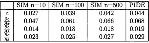
A.l Price of a call option with strike K = 50 in the Merton model 139 A.2 Vega of a vanilla call option in the Merton m o d e l ...140 A.3 Rho of a vanilla call option in the Merton M odel...140 A.4 Sensitivity with respect to changes in the jump intensity A of

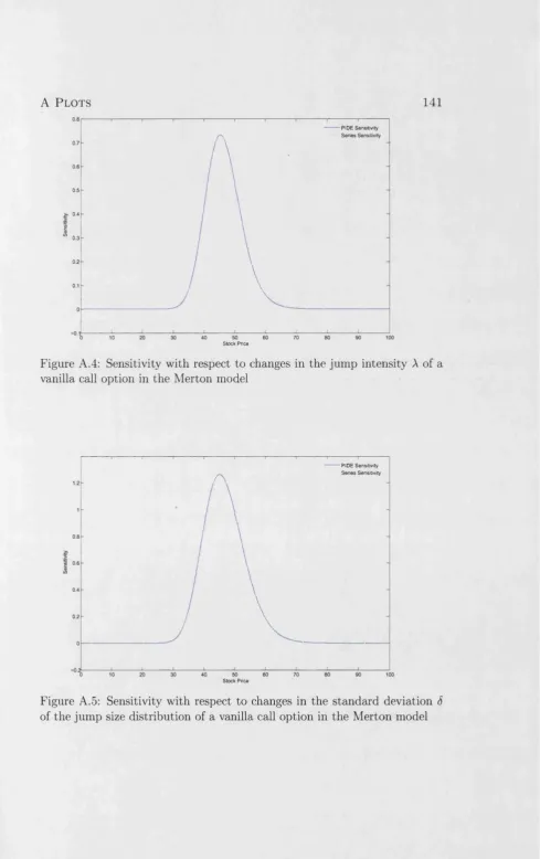
a vanilla call option in the Merton m o d e l...141 A.5 Sensitivity with respect to changes in the standard deviation

8 of the jump size distribution of a vanilla call option in the Merton m o d e l...141 A.6 Sensitivity with respect to changes in a of a vanilla call option

in the variance gamma m o d e l ... 142 A.7 Sensitivity with respect to changes in d of a vanilla call option

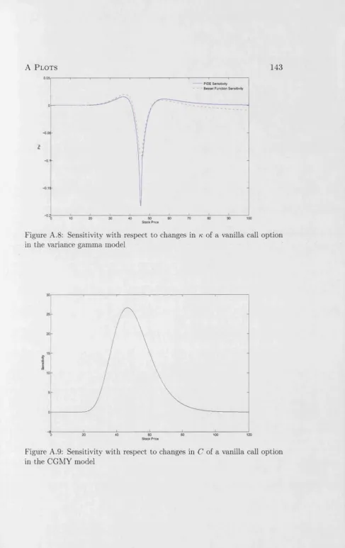
in the variance gamma m o d e l ... 142 A.8 Sensitivity with respect to changes in k of a vanilla call option

in the variance gamma m o d e l ... 143 A.9 Sensitivity with respect to changes in C of a vanilla call option

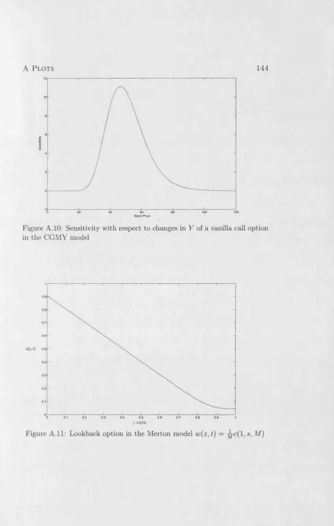
in the CGMY m o d e l ... 143 A. 10 Sensitivity with respect to changes in Y of a vanilla call option

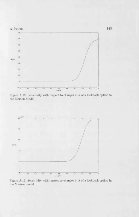
in the CGMY m o d e l ... 144 A.11 Lookback option in the Merton model w(z, t) = s, M) . 144 A. 12 Sensitivity with respect to changes in a of a lookback option

in the Merton M o d e l... 145 A. 13 Sensitivity with respect to changes in A of a lookback option

Li s t o f Fi g u r e s 9 A. 14 Sensitivity with respect to changes in 5 of a lookback option

in the Merton m o d e l ... 146 A. 15 Lookback option in the variance gamma model

v & t ) = m C( M , M ) ... 146

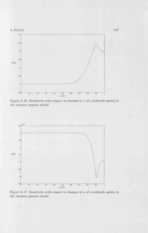
A. 16 Sensitivity with respect to changes in a of a lookback option in the variance gamma m o d e l ... 147 A. 17 Sensitivity with respect to changes in k of a lookback option

in the variance gamma m o d e l ... 147 A. 18 Sensitivity with respect to changes in 8 of a lookback option

in the variance gamma m o d e l ... 148 A.19 Asian option in the Merton model w(t, z) = J c(t, s, a ) 148 A.20 Sensitivity with respect to changes in A of an Asian option in

the Merton m o d el... 149 A.21 Sensitivity with respect to changes in a of an Asian option in

the Merton m o d el... 149 A.22 Exchange option v(t, z) = | c(t, s, s ) ... 150 A.23 Sensitivity with respect to changes in p of an exchange option

in the Merton m o d e l ... 150 A.24 Sensitivity with respect to changes in g of an exchange option

List of Tables

7.1 Price function and greeks for a lookback option with parame­ ters A = 0.1, a = 0.1, S = 0.1... 117 7.2 Price function and greeks for a lookback option with parame­

C hapter 1

Introduction and sum m ary

1.1

Introduction

1 In t r o d u c t i o n a n d s u m m a r y 1 2 process X t. Depending on the financial contract and the market under con­ sideration, various Levy processes have been put forward that can adequately represent price dynamics. In exponential Levy models option prices can be expressed as solutions to partial integro-differential equations for which we will throughout use the abbreviation PIDE.

We are interested in how sensitive prices of financial derivatives are to changes in the model parameters in a given model and to changes of the stochastic nature of the model. Knowledge of the sensitivities, in finance known as the greeks, is crucial to management of the risk of the financial contract. Most textbooks on mathematical fiance such as Bingham and Kiesel [4], Bjork [5], Hull [24], and Musiela and Rutkowski [32] have chapters on sensitivity analysis and the greeks. However, they only treat the case where the price function is given in a closed form. This is possible for a wide range of options in the Black-Scholes model. In exponential Levy models closed form solutions do not exist in general. When closed form expressions are out of reach one has to resort to numerical methods in order to obtain op­ tion prices and their sensitivities. Several numerical methods have been put forward to price options. The most prominent are simulation and (integro-) differential equation methods, but also Fourier transform methods and nu­ merical integration are being used. To obtain sensitivities simulation is most widely used.

1.2

Sum m ary

1 In t r o d u c t i o n a n d s u m m a r y 1 3 lowing this latter approach we first extend its use to a range of options in the Black-Scholes model and then apply this method to exponential Levy models where we solve a system of PIDE in order to obtain option prices and greeks. The dynamic PIDE approach is further extended to calculate sensitivities of option prices with respect to changes in the stochastic model of the underlying price process.

C hapter 2

S en sitiv ity analysis in finance:

th e greeks

The greeks of a price function tell us how much the price function changes if there are changes in the price of the underlying asset, changes in model parameters, or potentially in changes across families of parametric models. At first glance sensitivities with respect to changes in model parameters seem self-contradictory, since a model parameter is by definition a constant, and thus cannot change within a given model. The greeks with respect to changes in model parameters are therefore sensitivities with respect to misspecifica- tions of the model parameters. Greeks with respect to changes across families of parametric models are sensitivities with respect to misspecifications of the p.arametric model.

2 Se n s i t i v i t y a n a l y s i s in f i n a n c e: t h e g r e e k s 1 7

2.1

The Black-Scholes market and th e greeks

We consider the Black-Scholes market [6] with two basic assets, a risk-free one (typically a bond or a money market account) and a risky one (typically a stock). Under the risk neutral measure the prices of the two assets are given by

Bt = er\

S( = S0e H ? ) t+'’H\

where r is the risk-free interest rate, o the volatility of the stock, and Wt is a Brownian motion. Their dynamics under the risk neutral measure are given by the stochastic differential equations

dBt = Bt r dt,

dSt = St {r dt + a dWt).

The unique price c(t, St) at time t of a European style option with payoff h and maturity T is given by the risk-neutral valuation formula

c(t, St) = E[e~r<-T~i> h(Sr)\ F t l (2.1) where E is the expectation under the risk neutral measure and (FT)o<T<t is the filtration generated by the Brownian motion. Using Ito’s formula it can be shown that the price function c(t,s) = ’E[e~r ^r ~t^h(ST)\St = s] satisfies the Black-Scholes equation

ct(t, s) = r c(t, s) - rs cs(t, s) - 2s2 css(t, s), (2.2) for all (t, s) G [0, T) x (0, oo), subject to the terminal condition

2 Se n s i t i v i t y a n a l y s i s in f i n a n c e: t h e g r e e k s 1 8 where we have used subscripts to denote derivatives. For a European call

option the terminal condition is

c(T, s) = max(s — K, 0), s > 0.

For computational purposes it may be useful to add auxiliary boundary con­ ditions, which for a European call option are

c(t,0) = 0,

c(i, s) ~ s — Ke~r (T~t\ s —> oo.

While deriving differential equations we will often encounter the quadratic covariation [X, Y]t of two processes X t and Yt. For all processes we consider, the quadratic variation exists and is defined as

[X, y], = lim ] T ( X (i+1 - X k )(Yl w - Yti) in probability, (2.3)

1 1 ii€n

where we sum products of increments along the partition II of the time interval [0, £], letting the grid size go to zero. In case X t = Yt we call it the quadratic variation process.

2 Se n s i t i v i t y a n a l y s i s i n f i n a n c e: t h e g r e e k s 1 9 respect to the volatility, and 0 the sensitivity of c with respect to time:

dc ds' d2c ds2 ’ dc d r’

dc d a’ dc d t’

where c = c(t, s, <r, r) is a function of the initial stock price, time, and the model parameters. We now discuss several ways of calculating the greeks.

2.2

Classical approach based on closed from

expressions

The greeks of options that have a closed form price function can be obtained by simply differentiating the price function with respect to the underlying stock price value, time, and the model parameters. Solving the Black-Scholes equation (2.2) for an European call with strike K and maturity T yields

c(s,t) = s N { d1) - K e - r <:r- t) N(d2), A =

r = p =

V =

0 =

where

2 Se n s i t i v i t y a n a l y s i s in f i n a n c e: t h e Gr e e k s 2 0 The greeks for this option are

A = N(di), r = J W _

s a \JT — t ’

p = K ( T - t ) e - r^ N(d2),

V = s y / T ^ t N ' i d . ! ) , 0 =

where N(-) denotes the cumulative standard normal distribution and N'(-) its density. This approach works for many options in the Black-Scholes frame­ work such as for barrier options, lookback options, and exchange options, where the price function can be expressed in closed form. For Asian options this approach is not straightforward. The price of an Asian option can be expressed as a triple integral which is difficult to evaluate numerically, see Yor [42].

2.3

D ynam ic approach

2 Se n s i t i v i t y a n a l y s i s in f i n a n c e: t h e g r e e k s 2 1

2.4

M onte Carlo approach

Simulation has proved to be a valuable tool for estimating security prices for which simple closed form solutions do not exist. The estimation of sen­ sitivities presents both theoretical and practical challenges to Monte Carlo simulation. Following Broadie and Glasserman [8] and Glasserman [21] we present the most important methods for obtaining derivatives of security prices using simulation. In many cases the parameter with respect to which we want to calculate the price sensitivity can be seen as either a parameter of the payoff or a parameter of the probability measure. We illustrate this with a European vanilla call option. If all the parameters are assumed to be in the payoff function, the price function at time t is written as

\ 1 _ x2 0 1 , e 2 dx.

) V27T

If all the parameters are put in the probability measure, the price is written as

c(£, s) = e_ r(T_t) f maxfa: — K, 0)--- . —~—y=e ^ dx,

V ' 7 - o o x a y / T ^ t y / 2 ^

where

^ M ! ) - (»■ - S ) ( r - 0

d { x ) = ■

In the finite difference method the parameter of interest is assumed to be in the payoff function and the probability measure is fixed. This method goes as follows: Firstly, an initial simulation is run to determine the price of an asset. Secondly, the parameter of interest is perturbed and another simula­ tion is run to determine the perturbed price. The estimate of the derivative is the difference in the simulated prices divided by the parameter perturba­ tion. This method is easy to understand and implement, but since it involves simulating at two values of the parameter of interest it is computationally not very efficient. Moreover it produces biased estimates [21]. Consider a

2 Se n s i t i v i t y a n a l y s i s in f i n a n c e: t h e g r e e k s 2 2 European style option whose price depends on a parameter 9 and is given by

/

•OO

where h(8) is the discounted payoff. To estimate the derivative of c(9) with respect to 6 we simulate n independent replicates h\{9),. . . ,hn(9) at the parameter value 6 and n additional replicates h\{9 + d) , . . . , hn{9 + d) at the parameter value 6 + d for some d > 0. Then, we average each set of replicates to obtain h{9) = £ and h{9 + d) = £ S L i KiO + d). The form of the forward difference estimator of the sensitivity is then

h{9 + d) - h{9)

The bias of the forward difference estimator is dc(X,9) Bias(Aj?) = E A p

d9 o(d),

where we used Landau’s notation / = 0(g(d)), meaning

v f(d)

limsup - r - r < oo. d—*o g\d)

By simulating at 9 + d and 9 — d, we can form a central difference estimator h(9 + d) - h{9 - d)

A c = It has a bias of

Bias(Ac) = E Ar? — 2d

dc(X, 8)

d9 = 0 ( d 2).

2 Se n s i t i v i t y a n a l y s i s in f i n a n c e: t h e g r e e k s 2 3 expectation operator can be interchanged, one can write the sensitivity as

d

± E [ h ( X, 9)] = E

deKx,e)

/

— h{x\9)g{x)dx,

where h is the discounted payoff function and 9 is a parameter in the pay­ off. From the dominated convergence theorem we know that the inter­ change of differentiation and integration is allowed if the derivative ^ h{9) exists almost everywhere and there is an integrable function k(x) such that

\\{h{x] 6 + d) — h(x\9))g(x)| < k(x) for all x and d small enough. This is typically only true if the payoff function is uniformly continuous in the pa­ rameter of differentiation 6. The name of the method stems from the fact that the expression ^ h(0) is called the pathwise derivative of h at 9.

The likelihood method, like the pathwise method, involves simulation at only one parameter value and produces unbiased estimates. It puts the de­ pendence of the parameter of interest in the underlying probability measure rather than in the payoff function and hence does not require smoothness in the discounted payoff. We consider a discounted payoff h as a function of a random variable X and suppose that X has probability density g{x,9) where 9 is a parameter of that density taking values in R. To derive a derivative estimator, we suppose that the order of differentiation and integration can be interchanged and we obtain for the sensitivity

-^Eg[h{X)] =

J

g(x-,e)

= E„ \h{X)

g{x-,e)

J

where we have written g(x\ 9) for • Just 85 in the pathwise method this method is valid if the differentiation and integration can be interchanged. This is true if the derivative ^g{x\ 9) almost everywhere exists and the func­ tion |h(x)2(g(x] 9 + d) — g(x\ 0))| can be bounded by an integrable function k{x) for small enough x and d. As probability densities are typically smooth functions this is usually satisfied.

2 Se n s i t i v i t y a n a l y s i s in f i n a n c e: t h e Gr e e k s 2 4

not even continuous limits the scope of the pathwise method. In contrast, smoothness conditions are usually satisfied by the probability densities aris­ ing in applications of the likelihood ratio method. The main drawback of the likelihood ratio method is that it requires the explicit knowledge of the probability densities and that its estimates tend to have a large variance [21].

C hapter 3

D ynam ic sen sitivity analysis in

th e Black-Scholes market

3.1

European vanilla options

Throughout we will denote the interest rate by r, the strike price by K, and the volatility of the Brownian motion by a. Recall the Black-Scholes equation (2.2) for a European call option

ct(t, s) = r c(t, s) - rs cs(t, s) - ^ 2s2 css(t, s), (3.1) for (£, s) E [0, T) x (0, oo), subject to the terminal condition

c(T, s) = max(s — K, 0), s > 0, (3.2) and the boundary conditions

c(t,0) = 0, (3.3)

3 Dy n a m i c s e n s i t i v i t y a n a l y s i s i n t h e Bl a c k- Sc h o l e s m a r k e t 2 6 equation for the sensitivity p — :

pt(t, s) = r p(t, s) + c(t, s) - rs ps{t, s) - s cs(£, s) - ^<r2s2 pss(£, s), (3.5) for (t,s) G [0, T) x (0,oo), with the terminal condition

p(T, s) — 0, s > 0, (3.6)

and the auxiliary side conditions p{t,0) = 0,

p(t, s) = (T — t) e~r (T~^ K, s —► oo.

Similarly, differentiating with respect to the volatility a we obtain the PDE

and the auxiliary boundary conditions V(t,0) = 0,

V(t, s) = 0, s —► oo.

To determine the price function and its greeks, the system of PDE (3.1), (3.5), and (3.7) has to be solved subject to its terminal conditions (3.2), (3.6), and (3.8). One starts with the boundary condition at time t = T, specifying the known terminal values for the price function and the greeks in the state interval one has chosen to work in, and then works backwards in time calculating at each time step the option prices and the sensitivities. Doing so, one obtains the price and the sensitivities for a whole range of for V = £ :

V,(f, s) = r V ( t , s ) - rs Vs(f, s) - ^cr2s2Vss - as2 c,s(t, s), (3.7) for (t, s) £ [0, T) x (0, oo), the terminal condition

3 Dy n a m i c s e n s i t i v i t y a n a l y s i s i n t h e Bl a c k- Sc h o l e s m a r k e t 2 7 strikes and times to maturity. This method is called the dynamic approach.

3.2

Lookback options

Lookback options provide investors with the possibility to look back in time and exercise an option at the ideal time. Obviously this opportunity has its price and invariably lookback options are more expensive than their European counterparts. We write S t for the stock price process, Mt = sup0<T<t ST for its running maximum, and m t = inf0<r<t ST for its running minimum over the interval [0, t]. There are four basic types of lookback options. The two floating strike lookback options are, firstly, the call option with payoff

h(Sr, ttit) = St ~ ttit:

giving the right to buy at the low over [0,T], and secondly, the put with payoff

H(Stj Mt) — Mt — St^

giving the right to sell at the high over [0, T\. Floating strike lookback options are not options in a strict sense as they will always be exercised and hence the pricing reduces to finding the expectations of the running maximum E [ M r ] and the running minimum E [ r a r ] under the risk neutral measure. The two fixed strike lookback options are the call, with payoff

Ii(Mt) = max (M r — K, 0),

and the put, with payoff

h(m r) = max (A" — m r, 0).

The fixed strike prices are special cases of the functional E [ h ( r a r ) ] and E [ h ( M r ) ] . P D E approaches to lookback options can be found for exam­ ple in Wilmott [18] or Zhu [43]. In the Black-Scholes framework closed form solutions exist for the four standard lookback options presented above. The

3 Dy n a m i c s e n s i t i v i t y a n a l y s i s in t h e Bl a c k- Sc h o l e s m a r k e t 2 8 closed form solutions for the floating strike lookback options have been de­ rived in Goldman et al. [22]. The closed form solutions for the fixed strike lookback options have been derived in Conze and Viswanathan [17].

3.2.1

F lo a tin g strik e lookback p ut

We take the floating strike lookback put as an example and undertake to derive PDE governing its price and the greeks. We show two different ways how the state space can be reduced and a PDE in time and only one more variable can be obtained. The price of a floating strike lookback put option at time t is

c(t, St, Mt) = E[Mt - Srl-FJ,

where T t is the er-algebra generated by the Markov process (St, Mt). To derive a PDE for the price of the lookback option we apply Ito’s lemma to the discounted option price e~Tt c(t, St, Mt). Following Shreve [37] we obtain

d(e~rt c(t, St, Mt)) = e~rt ^ - r c(t, St, Mt) dt + c*(£, St, Mt) dt + cs{t, St, Mt) dSt + 2Css(^’ Mt)d[S, S']* + cm{t, St, Mt)dMt^j

= e~r t ( j ^ - r c(t, St, Mt) + ct (t, St, Mt)

-\-rSt cs(t, St, Mt) + Sf css(t, St , Mt)^j dt + crSt cs(t, St, Mt) dWt + cm(t, St, Mt) d M ^ j ,

3 Dy n a m i c s e n s i t i v i t y a n a l y s i s i n t h e Bl a c k- Sc h o l e s m a r k e t 2 9 the PDE

Ct(t} s, m) + ^<r2s2css(t, s, m) + rs cs(£, s, m) — r c(t, s, m) = 0, (3.9) for t G [0, T) and 0 < s < m < oo, subject to the terminal condition

c(T,s,m) = m — s. (3.10)

For the first auxiliary boundary condition we investigate the option price when the stock price is close to zero and obtain

limc(£, s,ra) = m e _r^T_^. (3.11)

s—+0

To obtain the second auxiliary boundary condition we use the fact that cm{t,Su Mt)dMt must be zero. The term dMt is zero when St < Mt. How­ ever, at the times when Mt increases, this is when the stock price is equal to its running maximum, cm(£, St, Mt) must be zero for cm(t, St, Mt) dMt to vanish. This gives us

C m ( t , s , m )|a=m = 0. (3.12)

Due to the special form of the payoff function (3.10), equation (3.9) and its side conditions can be transformed and written in new coordinates using c(t ,s ,m) = mw(t,£) where £ = Doing so, both the PDE and the side conditions only depend on time and the state variable £ = The derivatives of the price function in the transformed coordinates are

ct(£, s,m) = m w t(t, £), cs( t, s ,m) = Wf(t,£), css(t, s, m) = -j-iuK(t,£). In the transformed coordinates the PDE is

3 Dy n a m i c s e n s i t i v i t y a n a l y s i s in t h e Bl a c k- Sc h o l e s m a r k e t 3 0 for (tj£) € [0, T) x (0,1). The boundary conditions for w(t, £) can be obtained from the boundary conditions (3.10), (3.11), and (3.12) of c(t,s,m). In particular,

m — s — c(T, s, m) = m w(T, £) implies

Furthermore,

m e~r (T-t) _ c(^ o, m) = m w(t,0) implies

w(t,0) = e~r (T~t\

and finally

0 = cm(t, s, m)\s=m = w(t, 1) - wz(t, O k -i implies

^ ( t ,0 k=i = w (t , l ).

We now calculate the greeks using the dynamic approach. As the PDE for the lookback option and the vanilla option differ only in the side condition, the same goes for the PDE for the greeks. Differentiating equation (3.13) with respect to the interest rate we obtain a PDE for g =

et{t, 0 + ^ 2£2Qttfa 0 + f r wdt> t ) ~ r e(t, 0 - w ( t , f) = o, (3.14) for (t, f) 6 [0, T) x (0,1) with terminal condition

3 Dy n a m i c s e n s i t i v i t y a n a l y s i s i n t h e Bl a c k- Sc h o l e s m a r k e t 3 1 and auxiliary side conditions

e«(*.?)l£=i = e(t,

1)-Differentiating (3.13) with respect to the volatility, we obtain a differential equation for v =

+ i r v ( (t,(.) — rv(t,£) = 0, (3.15) for (t,() 6 [0, T) x (0,1) with terminal condition

u(T,O = 0, and auxiliary side conditions

v(t,0) = 0, v*(*,f) le=i = v(t,1).

Solving the system of equations (3.13), (3.14), and (3.15) with the appropri­ ate side conditions and transforming the variables w, p, and v back to c, p, and V, using

c(t, s,m ) = mw(t,£), p{t,s,m) = mg(t,£),

V(t, s, m) = m v ( t, £),

we obtain the price and the greeks for the lookback put.

3 Dy n a m i c s e n s i t i v i t y a n a l y s i s in t h e Bl a c k- Sc h o l e s m a r k e t 3 2 from the closed form expression as derived in [32]:

2 c(s, t) = - s N ( —di) + m e - 'M N ( - d 2) + s N(di)

2 r

«3‘6>

In (A) + (r ± |<t2) (T - t) di,2 —

(T y/T — t

The greeks in the closed form approach are then obtained by differentiating (3.16).

3.2.2

A m artin gale m eth o d

We now give an alternative derivation of the option price defining PDE baaed on a martingale technique. Consider the martingale

Mt = E[Mt - ST\ f t],

where St is the stock price process and Mt = sup0<T<tST is its running maximum. The martingale can be written as

Mt = E m axv(Mt,S t sup

" t < r < T

= St f ( t , Q t), with

3 Dy n a m i c s e n s i t i v i t y a n a l y s i s i n t h e Bl a c k- Sc h o l e s m a r k e t 3 3 and

r n \ urT ( ( r - £ ) T + c T W T\ ( r - d ) ( T - t ) + a ( W T - W t )

f{t,q) = E max I g, sup 2 / I — eV 2 ' L V 0 < r < T - t )

(3.17) Using Ito’s lemma we obtain the dynamics of

Qt-dQt = j - dMt - ^ dS, + d[S, S]t, which can be written as

dQt = Qt( - r dt - ad W t + a 2 dt), Qt > 1. The dynamics of the martingale Mt are

dMt — dSt f ( t, Qt) + St ^ft(t, Qt) dt + f q(t, Qt)dQt + 2 ^ " ^ ’ ^1*) fq(t, Qt)dQt,

= ■?( ( /t( i, Qt) + r / ( i , Qt) + ~<7^Qj /„(<, Q,) - r Q, /,(«, Q,) J dt

+ St a f ( t , Q t)dWu (3.18)

where we used d[Q, Q]* = Q2 a2 dt. Setting the drift term in equation (3.18) to zero one obtains the PDE

ft(t, q) + r f ( t, q) + ^ a 2q2 f qq(t, 9) - rg /,(£, g) = 0,

valid for (t,q) £ [0,T) x (l,oo). The terminal condition in this parametrisa- tion is

3 Dy n a m i c s e n s i t i v i t y a n a l y s i s i n t h e Bl a c k- Sc h o l e s m a r k e t 3 4 If the stock price goes to zero then we obtain the first auxiliary boundary condition

f{t,q) = q - e r{T~t\ q -> oo.

We obtain the second auxiliary boundary condition by inspecting equation (3.17). If the stock price is at its maximum then q = 1. Because of the diffuse nature of Brownian motion the second term in the maximum function in (3.17) is always bigger than 1. Therefore, f(t,q) does not explicitly depend on q at q = 1. This leads to the second auxiliary boundary condition,

f q(t,q) |,=i = 0. The price function of the option is then

p(s,t) = e~r{-T~t) sf(t ,q) .

3.3

A sian options

Asian option is a generic name for the class of options whose terminal payoff depends on the average value of the underlying asset during some period of the option’s lifetime. In contrast to standard options, Asian options are more robust against manipulation near their expiry dates. Asian options are widely used in practice, for instance, for commodities and in foreign exchange markets. The two major types of Asian options are floating strike Asian

3 Dy n a m i c s e n s i t i v i t y a n a l y s i s in t h e Bl a c k- Sc h o l e s m a r k e t 3 5 number called the strike price. There also exist more general Asian options with payoffs such as At — K\ St — 0), where Ki and K 2 are two fixed numbers.

3.3.1

F lo a tin g strik e A sian op tion s

We consider a floating strike Asian call option. The price of such an option is given as the expected discounted payoff under the risk neutral measure

Using Ito’s formula one can show that in the Black-Scholes model the price function

valid for (t, s, a) G [0, T) x (0, oo) x [0, oo) subject to the terminal condition

This is just the Black-Scholes equation for a vanilla option with the addi­ tional term ca(t, s, a), taking into account that the option also depends on an average price of the underlying asset over a certain time period. PDE methods for a wide range of exotic options can be found in Zhu [43]. Follow­ ing [25], [36], and [18] we show, that the state space of equation (3.19) can be reduced and a PDE in only two variables can be obtained. Alternatively one can use a martingale method to directly derive a price determining PDE that only depends on time and one further variable. We will present the martingale technique in the next section as it works for both fixed strike and floating strike Asian options.

c(t,Su At) = e~r ^ E max 5t - - A t ,0 1_ T t . T

c(t,s,a) = e r (T max ( St

is the solution to the PDE

3 Dy n a m i c s e n s i t i v i t y a n a l y s i s i n t h e Bl a c k- Sc h o l e s m a r k e t 3 6 To reduce the state space we use the ansatz c(t,s,a) = sh(t,q) with

X 9l T s'

q = h - . The derivatives of the price function in the new coordinates are Cf(t,s,u) = sht(t,q),

cs(t, s, a) = h(t, q) - q hq(t, q), Q^

Css(t> = hqqipi

ca(t,s,a) = 7f,hg{t,q). (3.20)

Inserting (3.20) into (3.19), we obtain

ht(t,

q)

h(T, q) = max(l — g, 0).

For computational convenience we introduce the auxiliary boundary condi­ tions as outlined in [18]. When Qt = is very large the probability that the stock price at expiry is greater than the average over T goes to zero:

lim P

q—*oo

Qt

q

and the option expires worthless. This gives us the first auxiliary boundary condition

h(t, q) = 0, g —> oo.

3 Dy n a m i c s e n s i t i v i t y a n a l y s i s in t h e Bl a c k- Sc h o l e s m a r k e t 3 7 leads to a contradiction. By Assumption, the term g2hqq{t, q) is bounded:

Integrating twice we see that this means h(t, q) = 0(\ogq). For small q this contradicts the fact that h(t, q) is bounded. We therefore conclude that

\im q2hqq(t,q) = 0,

and equation (3.21) reduces for q —► 0 to the second boundary condition ht(t,0) + ^ h q(t,q)|g=0 = 0.

Using the dynamic approach, the greeks can easily be calculated. Differ­ entiating (3.21) with respect to the interest rate r, using P — % = and k = one obtains the PDE for A:,

h{t, q) + ^cr2q2 kqq{t, q) + - rq^j kq(t, q) - q hq(t, q) = 0, (3.22) valid for (t, g) E [0, oo) x [0, oo) with the terminal condition

k(T ,q) = 0, and auxiliary side conditions

' k(t, g) = 0, q —> oo,

fct(i,0) + i/cg(^g)|g=o = 0.

Differentiating (3.21) with respect to the volatility cr, using V = = s|£ and Z = one obtains the PDE for Z

3 Dy n a m i c s e n s i t i v i t y a n a l y s i s i n t h e Bl a c k- Sc h o l e s m a r k e t 3 8 valid for (t, q) G [0, oo) x [0, oo) with terminal condition

and auxiliary side conditions

l{T,q) = 0,

l(t,q) =0, q-+ oo, lt (t,0) + — lq(t, <z)|g=0 — 0.

Then the system of equations (3.21), (3.22), and (3.23) has to be solved with respect to the relevant terminal and side conditions. Finally, the variables h, A;, and I have to to transformed back to c, p and a.

3.3.2

F ix ed strike A sian op tion s

Rogers and Shi [34] showed that not only for floating strike but also for fixed strike Asian options the state space can be reduced. Hence, the problem reduces again to solving a parabolic PDE in two variables. We derive the PDE for the fixed strike Asian call option with payoff max(^ At — K, 0) using a martingale technique. Consider the martingale

Mt = E max Tt

= St E = St h{t,Qt),

( t In St dr h f T ST dr K '

^ [ z A s ^ + z A s t S i- 0

where

Qt

—

3 Dy n a m i c s e n s i t i v i t y a n a l y s i s in t h e Bl a c k- Sc h o l e s m a r k e t 3 9 and

h(t, q) = E max q -1- k i t Sr <lT

S, ,0 (3.24)

We have essentially split the payoff into a part which only depends on the past and a part which only depends on the future. To see this we write

/ (T STdr _{J * e ^ - x ) (’--*)+"0vr-w,)dT}

which does not involve anything from the sigma-algebra T t and hence, be­ cause of the independence of increments, is independent of F t. Using Ito’s formula we obtain the dynamics of Qt:

dQt = Qt{~r dt - a dWt + a2 dt) + ^ dt.

We can then apply Ito’s formula to the martingale Mt to obtain its dynamics dMt = dSt h(t, Qt) + St dh(t, Qt) + dSt dh(t, Qt)

= St(r dt + a dWt) h(t, Qt)

+ St ^ht(t, Qt) dt + hq(t, Qt) ^Qt( - r dt - a dWt + a2 dt) + Tpdt'j + ^hqqit, Qt) dt^j - cr2 StQthq(Qt, t) dt.

Setting the drift term to zero, we obtain a P D E for h:

ht(t, q) + r h(t, q) + ^a2q2 hqq(t, q) + Q ; - rq^j hq(t, q) = 0, (3.25)

valid for (t,q) G [0, T) x (—0 0,0 0). Equation (3.25) has to be solved subject to the terminal condition

3 Dy n a m i c s e n s i t i v i t y a n a l y s i s i n t h e Bl a c k- Sc h o l e s m a r k e t 4 0 Introducing

f(t,q) = e_r(T_t)/i(t,g) equation (3.25) can be simplified to

ft(t, <l) + \ /w(*> ?) + Q ; - rq j f q(t, q) = 0, (3.26) valid for (t, q) E [0, T) x (—0 0,0 0) with the terminal condition

f(T,q) = max(<7,0), and the auxiliary side conditions

f ( t , q ) = 0, q - > -00

1 1 _ p - r ( T - t )

/ ( t , g) = e - ’'<T- t>g + - --- , ? > 0.

1 r

3 Dy n a m i c s e n s i t i v i t y a n a l y s i s in t h e Bl a c k- Sc h o l e s m a r k e t 4 1 and one can explicitly calculate the price of the option. The option price function at time t = 0 can be written as c = s /(0, — y )• The same martingale technique can be applied to a floating strike Asian option and one obtains the PDE (3.21). Note that apart form having different side conditions the PDE for the fixed strike Asian option (3.26) and the PDE for the floating strike option (3.21) are the same. To obtain the greeks we use the dynamic approach and derive their corresponding PDE. p is obtained via p(0, s) = sg(0, -^- ), where g = is given by the PDE

9t(t, q) + i a2q2 gqq{t, q) + - q'j gq{t, q) - q f q(t, q) = 0,

valid for (t,q) G [0,T) x (—0 0,0 0) with terminal condition g(T, q) = 0,

and the auxiliary boundary conditions g{t,q)= 0, q —» —0 0,

9 { t ' q ) = T

7

t)e"r(T' ‘,<7

The greek V is given by V(0, s) = sw (0, —y ), where w = satisfies the PDE

wt(t, q) + ^ a 2q2 wqq(t, ?) + Q ; “ wg(*, q) + aq2 f gq(t, g) = 0, valid for (t,q) G [0,T) x (—00,0 0) with terminal condition

w(T, q) = 0 , and the auxiliary boundary conditions

3 Dy n a m i c s e n s i t i v i t y a n a l y s i s in t h e Bl a c k- Sc h o l e s m a r k e t 4 2

3.4

Barrier options

Barrier options are options where the payoff depends on whether the price of the underlying asset reaches a certain barrier level B during a certain period of time. There are four basic types of barrier options. Down-and-out options are similar to vanilla options, but they have the additional feature that they cease to exist if the stock price hits a barrier level B < So and nothing is paid to the holder of the contract. Up-and-out options cease to exist if a barrier level B > Sq is reached. Up-and-in options only come into existence if a

barrier B > So is hit during the lifetime of the option. Down-and-in options only come into existence if a barrier B < So is hit during the lifetime of the option. The prices of the ’in’ options can be obtained by calculating the price of the corresponding vanilla option and the corresponding ’out’ option and the using the fact that the price of the ’in’ option must be equal to the price of the vanilla option minus the price of the ’out’ option. Many other types of barrier options have been developed. These include moving-boundary options where the constant barrier is replaced by a stochastic process, Asian barrier options, and options where the barrier only applies to a certain part of the time-interval. For the standard barrier options closed form solutions for the price exist in the Black-Scholes model. Many of the more exotic barrier options can easily be implemented with the PDE approach, and since usually no closed form solutions exist, this is the only possible analytic approach.

3.4.1 D ow n -an d -ou t call

As an example we explain how a down-and-out call option and its greeks can be priced. Both the dynamic and the closed form approach to calculate the greeks for a down-and-out option are explained in Norberg [33]. The price function of such a down-and-out call option at time t is

cDO(t,s) = e- ’-(r - ‘)E[(Sr - = «]•

3 Dy n a m i c s e n s i t i v i t y a n a l y s i s i n t h e Bl a c k- Sc h o l e s m a r k e t 4 3 PDE

ct(£, s) = r c(t, s) - rs cs(t, s) - css(t, s), (3.28) for £ G [0, T) and 0 < s < B, subject to the natural side conditions

c(£, B) = 0,

c(T, s) = max(0, s — K), and the auxiliary side condition

c(t, s) ~ s — Ke~r (T~t\ s —> oo.

The greeks can be obtained by differentiating the defining PDE (3.28) using the dynamic approach. Doing so, we obtain the same equations as for the vanilla call option except for the additional barrier condition that the payoff is zero once the barrier has been hit. There exists a closed form expression for the price of a down-and-out call [32]. If the barrier level B is smaller that the strike K then the option price is given by

t, ^ ) , (3.29) where

CBs{t, s) = s N(di(t, s)) - e_r(T_f) K N(d2(t, s)),

and N(-) is the cumulative normal distribution. If the barrier level B is bigger that the strike then the option price is given by

CDo{t, s, B) = cBs{t, s) - ( — ~7~1

n

C-BS

CDo(t,s) = sN(xi) - K N {x2)

/ n \ +1 / rj \ —1

3 Dy n a m i c s e n s i t i v i t y a n a l y s i s i n t h e Bl a c k- Sc h o l e s m a r k e t 4 4 where

l n ( * ) + ( r ± £ ) ( T - t )

Xl

'2

a j T = i

M D + ^ t ) (T - i )

Vl'2 = ---T j r * ---■

Differentiating equation (3.29) or (3.30) with respect to the parameters in question we obtain the corresponding greeks.

3.5

N um erical results

The systems of PDE of this chapter can efficiently be solved using finite differences. A finite difference solver for PIDE is explained in detail in chapter 7. As the finite difference solver for PDE is a special case of the finite difference solver for PIDE we refer to chapter 7 for the technicalities and only report the numerical results here.

C hapter 4

E xponential Levy m odels

4.1

L evy processes and exponential Levy m od­

els

As we want to apply, in the next section, the dynamic sensitivity method to models with jumps, in particular to exponential Levy models, we first state some facts about Levy processes and about exponential Levy models. The properties about Levy processes are drawn from Sato [35]. We begin with the definition of a Levy process. A stochastic process X t is a Levy process if the following statements are satisfied:

1. X t has independent increments: For any choice of n > 1 and 0 < to < t\ < • • • < tn, the random variables X to, X tl — X to, • • • , X tn — Xtri_1 are independent.

2. X t has stationary increments: The distribution of X s+t — X t does not depend on t.

3. X t is stochastically continuous: Ve > 0 lim ^ o P{\Xt+h ~ X t \ > e) = 0. 4. Xo = 0 a.s.

4 Ex p o n e n t i a l Le v y m o d e l s 4 6 whose size is in the Borel set A C R bounded away from zero

v d t h h ] , A) = G [^1,^2] : AX* G A}.

The Levy measure v(A) of X t is defined as the expected number of jumps of X t per unit time interval whose size is in the Borel set A bounded away from zero

i / ( i 4 ) = E [ # { 4 G [ 0 , 1] : A X t eA}].

The Levy measure v is a positive measure in R. Its density (if it exists) need not be integrable and may exhibit a singularity at 0. It has the following properties

1. i/(T) < 00 if T is a Borel set bounded away from zero. 2. x 21/(dx) < 00 and ^({0}) = 0.

The Levy-Ito decomposition states that any Levy process Xt can be writ­ ten as

X t = j t + a B t + / x/j,(ds:dx)

J(o,t]x( R\(-i,D)

+ lim I x (p(ds, dx) — v{dx)ds), £_*° *Ao,t]x([—1,—e)U(e,l])

which is the sum of a drift, a Brownian motion, a term comprising large jumps, and a term comprising compensated small jumps.

The characteristic function of a Levy process X t has the so called Levy-Khinchin representation

a 2 2 ro c

E[e“ *‘] = e^W, ^{z) = ----— + iy z + (eizx - 1 - * z i l w<i) v[dx),

“ J — OO

(4.1)

4 Ex p o n e n t i a l Le v y m o d e l s 4 7 characterised by the triplet (7, <r2,^), hence called the characteristic triplet. A Levy process X t with characteristic triplet (7, a2, v) is said to be of

1. type A if a2 = 0 and u(M) < 0 0. The process X t is then of compound Poisson type.

2. type B if a2 = 0, i/(R) = 0 0, and Jjx|<:l |a;| 1'(dx) < 0 0. The process X t is then of finite variation and infinite activity, which means that its jumping times are dense in R+.

3. type C if either a2 > 0 or |ar| v(dx) = 0 0. The process X t is then of infinite activity and unbounded variation.

In exponential Levy models, the stock prices are given as an exponential of a Levy process Xt,

St = S0ert+X‘.

A good introduction to exponential Levy models can be found in Cont and Tankov [14]. The discounted stock price process So eXt has to be a martingale under some risk neutral measure. This can be achieved by imposing the following conditions

2 p

7 + y + / ( e 2 : _ 1 _ :rlNI<i) v (dx) =

4 Ex p o n e n t i a l Le v y m o d e l s 4 8 a Brownian motion part and a finite activity jump part or a infinite activity jump part but no diffusion part. The former models are called jump-diffusion models. However, Brownian motion can be obtained as the limit of an in­ finite activity process and is thus essentially included in pure jump infinite activity models.

4.2

Jum p-diffusion m odel

In jump-diffusion models the evolution of a stock price is given by the sum of a Brownian motion and a process that has a finite number of jumps in each finite time interval, representing rare events such as crashes. We restrict ourselves to the Merton jump-diffusion model [30], where the stock price is driven by the sum of a Brownian motion Wt and a compound poisson process where Nt is the Poisson process counting the jumps of X t and YJ are normally distributed random variables representing the jump sizes:

N t

X t = y t + a W t + Y , Y i ,

i=l

St = S0ert+X‘,

Y t - N i f i J 2).

The drift parameter 7 is chosen such that the discounted stock price process St = e~rt St = eXt is a martingale under some risk neutral measure. In this model the Levy measure is given by

4 Ex p o n e n t i a l Le v y m o d e l s 4 9

4.3

Variance gam m a m odel

The variance gamma model [29] is a pure jump model with infinite activity and finite variation. This model permits a good description of the volatility smile observed in option pricing at all maturities and for a wide variety of underlying assets. It has therefore become very popular within the finance community. The model is based on the variance gamma process

Yt = e z t + cjwZt,

(4.3) which is obtained by subordinating a Brownian motion with drift to a Gamma process Zt. Hefe a is the volatility of the Brownian motion and 6 is the drift of the Brownian motion. The density function / of the gamma distribution r(a,/?) is

f(x\ a, (3) = x a~l ~ e~ - , for x > 0, r ( a )

where T is the Gamma function, a is called the shape parameter, and (5~l is a scale parameter. We choose the parameters a = £ and P = \ to obtain a gamma process with mean t and variance nt. The variance gamma process has the particularly simple characteristic function

K ( z ; t, e, a ,«) = E(e*sY‘) = “ . The stock price process is given by

4 Ex p o n e n t i a l Le v y m o d e l s 5 0

is such that eXt is a martingale under some risk neutral measure. The random variable X t has the density

t i

p(x,t) = eAx C(t) |x|« 2K t _ i(B|a:|), K 2

where K n(x) is the modified Bessel function of the second kind,

A = - ₉₃

a1

yjd2 +2cr2/K, D = --- .

C(t) = 2(\/2nKttK<jY(t/k)) (2(j2/k, + 62)* 2«.

The modified Bessel function of the second kind K n{x) is one of the solutions to the PDE

+ x i ~ (x 2 + n 2 ) y=0 > and can be expressed as the integral

r ( n + i ) ( 2 x ) n r ° cos(«) K n{x) = {n + f - { X) (

V n Jo0 (t 2 - \ - X 2) n + 2Y<it.

More on Bessel function can be found in Abroamovitz [1]. The fact that the density of the process X t at time t is known as a function of a Bessel function will allow us to compute the price function of an option in the variance gamma model using numerical integration and to compare this results with the ones obtained using the dynamic PIDE approach. The Levy measure of this model is

v(dx) = - ^ -. eAt~B^ d x . (4.4)

k\x\

4 Ex p o n e n t i a l Le v y m o d e l s 5 1

4.4

Carr G em an M adan Yor (C G M Y ) m odel

In [9] a new model for asset returns is investigated. It is named the (CGMY) model after the authors Carr, Geman, Madan, and Yor and contains the variance gamma model as a special case. This model allows for the jump

tivity and variation, depending on the choice of the parameters. The authors conclude in their empirical study that most equity prices are best described by pure jump processes of infinite activity and finite variation. The stock return driving process X t is, not surprisingly, called the CGMY process. This process is a generalisation of the variance gamma process and a special case of the tempered stable process. Unlike in the variance gamma model, how­ ever, the density of the process X t at time t is in general not known in terms of some special function of mathematics. The Levy density of the CGMY process X t is given by

where C > 0, G > 0, M > 0, and Y <2. The condition Y < 2 is induced by

of 0. In the case Y = 0 the CGMY model reduces to the variance gamma model. In the case Y < 0 the process X t has finite activity. The parameter C may be viewed as a measure of the overall level of activity. The parameters G

side respectively of the Levy density. The parameter Y characterises the fine

infinite activity and variation. The stock price under the CGMY model is component of the asset return driving process to display finite or infinite

ac-(4.5)

the requirement that the Levy densities integrate x 2 in the neighbourhood

and M control the rate of exponential decay on the positive and the negative

structure of the process and determines whether the process is of finite or

St = S0e ^ u)t+Xt

where r is the interest rate and

4 Ex p o n e n t i a l Le v y m o d e l s 5 2

is such that e rtSt is a martingale under some risk neutral measure. The characteristic function (J)cgmy of the CGMY process is

(pCGMY = E[eiuXt] = etCT{-Y)((M-iu)y-My+(G+iu)y-Gy)

C hapter 5

O ption prices and greeks in

exponential Levy m odels

5.1

European vanilla options

5.1.1

D erivation o f th e P ID E

To start with we show how in exponential Levy models the price of an option can be expressed as a solution to a PIDE. Throughout we assume that the underlying stock price is given by an exponential Levy process which has the representation St = So ert+Xt, where X t is a Levy process with characteristic triplet (cr, 7, v) and r stands for the interest rate. The dynamics of the stock price process are given by

/

■OO

where Wt is the Brownian motion part, fi(dt, dx) is the jump measure, and v(dx) is the expected number of jumps in dx in a unit time interval. The integral term in (5.1) therefore represents a possible jump in the stock price process minus its expected value. The price of a European vanilla option at time t with payoff h on this stock is

5 Op t i o n p r i c e s a n d Gr e e k s i n e x p o n e n t i a l Le v y m o d e l s 5 4 Due to the independent increment property of Levy processes the conditional expected value in equation (5.2) can be written as

E[M Sr)l

H

ElHst

H

= K ( t , S t),

where K(t,u) = M[h(uer ^r~t^+XT~Xi)] = E[h(u5V-t)]- As St is the only relevant state variable, conditioning on the filtration (^>)o<r<t is the same as conditioning on St and we can write (5.2) as

c{t,St) = e_ r^r_ t'E [h(5r)|5(]. The discounted option price

c(t,St) = e -r i c(t,St) (5.3)

is a martingale. We want to apply ltd’s lemma to the discounted option price. The following condition assures that the option price function is smooth enough for Ito’s formula to make sense, see [35] and [14]. If

a > 0 or 3 /? e (0 , 2), s.t. lim infe-/3 f \x\2v(dx) > 0, (5.4)

£-+° J - e

5 Op t i o n p r i c e s a n d Gr e e k s in e x p o n e n t i a l Le v y m o d e l s 5 5 sufficiently differentiable and we apply Ito’s formula to equation (5.3) to obtain the dynamics of the discounted option price

dc(t, St) = — re~Ttc{t, St. ) dt + e~rt dc(t, St. )

= e~rt ^ - rc{t, St. ) dt + ct{t, St. ) dt + cs(t, St. ) dSt + \ c , s(t,St-)d[S,S]i

+

J

where [S, is the continuous part of the quadratic variation [S, S]t defined in equation (2.3). Dividing the dynamics into a drift and a local martingale part and using the fact that E[fi(dt,dx)\ = v(dx)dt, we obtain

dc{t, St) = e~rt ^ - rc{t, St. ) + <*(*, St. ) + rSt. c s(t, S’*.) + ^ S 2_a2c„(t, St-)

+

J°°

+ J

We now show that if

M>i the local martingale part

[ exv(dx) < oo, (5.5)

J lil> i

dMt = o St- cs(t, St-) dWt

5 Op t i o n p r i c e s a n d Gr e e k s in e x p o n e n t i a l Le v y m o d e l s 5 6 is actually a true martingale. Prom Sato [35] we know that

j ex v(dx) < oo <=> E [eXt] < oo,

J|x|>l|x|>l which in turn implies that

"t roo

E

r t roo

/ / (ex — 1)(fi(dx,dr) — ly(dx)dr)

JO J —oo

< 0 0.

Since the payoff function is Lipschitz, the price function c(t, s) is also Lips- chitz with respect to the stock price value

\c(t,sex) - c ( t , s)| < |s{ex - 1)|, which implies that

»t roo

E

r i roo

/ / (c(t, s ex) — c(t, s))(fi(dx, dr) — v(dx)dr)

J o J —oo

< 00,

and that Mt is a true martingale. Thus, the coefficient in front of a{t) has to be zero almost surely and it has to be zero for all possible values of St. This leaves us with the PIDE for the price function,

ct(t, s) + rs cs(t, s) + ^ a 2s2 css(t, s) - r c(t, s)

/

v(dx) (c(t, sex) — c(t, s) — (ex — l)s cs(t, s)) = 0, (5.6)

■OO

valid for (£, s) G [0, T) x (0, oo), subject to some terminal condition. For a European vanilla call option the terminal condition is

c(T, s) = max(s — K, 0), (5.7)

5 Op t i o n p r i c e s a n d Gr e e k s in e x p o n e n t i a l Le v y m o d e l s 5 7 computational purposes is necessary to add the boundary conditions

c{t,0) = 0,

c(t, s) ~ s — K e~r^T~t\ s —► oo.

In order to facilitate the numerical computations later on, we perform the change of variables as shown in Cont [16]:

t = T — t,

2/ = ln ( ^ ) + r r , and define new functions n(r, y) via

c(t,s) = e~rT K u(r,y). (5.8)

The derivatives of the price function in the new coordinates are c«(t, s) = e~rT K (r u(r, y) - uT(r, y) - r u„(r, y) ) , cs(t,s) = e~rT — uy(r,y),

css(t, s) = e~rT^ (uyy(r, y) - uy{r, y)), (5.9) and the shifted option price becomes

c(t, s ex) = e~rT Ku(t, y + x). (5.10)

5 Op t i o n p r i c e s a n d Gr e e k s i n e x p o n e n t i a l Le v y m o d e l s 5 8 valid for (r, y) G (0, T] x (—0 0,0 0), subject to the initial condition

w(0, y) = max(0, ey — 1), and the auxiliary boundary conditions

u { r, y ) = 0, y -> - 0 0, u(t, y) ~ ey — 1, y —> 0 0.

The fact that there are only linear functions in the argument of u(r, y) will later on simplify the numerical computation of the PIDE as it will allow us to evaluate it with finite difference methods on a grid with constant grid size.

5.1.2

G reeks in th e jum p-d iffu sion m od el

In order to obtain the sensitivities we differentiate equation (5.11) with re­ spect to the parameters in question. To start with we calculate V,