Observer based robust control

information.

Author(s): Dodds, Stephen J. Title: Observer based robust control Year of publication: 2007

Citation: Dodds, S.J. (2007) ‘Observer based robust control’Proceedings of Advances in Computing and Technology, (AC&T) The School of Computing and Technology 2nd Annual Conference, University of East London, pp.151-159 Link to published version:

OBSERVER BASED ROBUST CONTROL

S J Dodds

School of Computing and Technology, Control Research Group [email protected]; [email protected]

Abstract: This paper presents an original contribution to the field of robust control. Plant order uncertainty as well as parametric uncertainty is catered for while guaranteeing not only closed loop stability but also a precisely prescribed closed loop dynamic response to the reference inputs. The method extends to nonlinear multivariable plants. Its ability to control plants having different orders

without adjustment and yielding the same closed-loop dynamics is demonstrated by simulation of its application to speed control and position control of a permanent magnet synchronous motor drive. The model of the plant used in the observer can simply be a chain of integrators driven by each control variable, at least equal in number to the rank of the plant with respect to the associated controlled output. The controller is simple, requires no adjustment and requires little more computational power than a typical classical PID controller.

1. Introduction

Observer based robust control (OBRC) is a new control technique, applicable to linear or nonlinear uncertain plants subject to unknown disturbances, that achieves robustness according to the following definition:

The robustness of a control system is defined as its ability to produce a specified closed loop dynamic response to reference inputs, within acceptable error tolerances for the application in hand, despite a) uncertainties in the assumed plant model used for the control system design and b) unknown external disturbances.

By a specified closed loop dynamic response is meant the output response to a given reference input determined by a specified differential equation. The error tolerances are included to allow acceptably small departures from the ideal closed-loop response.

By an ‘uncertain plant’ is meant a plant whose mathematical model is not known

accurately: In addition to lack of accurate knowledge of the plant parameters, the uncertainty may also be in the plant order. OBRC superficially resembles internal model control (IMC) developed principally for the process control industry and later modified to cater for unstable plants (Yamada, 1999). There may be theoretical links between them, but the underlying strategies are different, IMC being formulated using transfer functions and therefore restricted to linear plants, while OBRC is formulated in the time domain and extends to nonlinear, multivariable plants. Also the block diagram structures presented in this paper are different from those of IMC.

will be given.

2. Underlying Concepts

2.1. Plant model mismatch equivalent input.

The applicability of the OBRC method depends on the existence of a plant model mismatch equivalent input, u_e, the meaning of which is defined in Fig. 2.1.

Fig. 2.1: Plant model mismatch equivalent input.

2.2. Theory of OBRC.

Consider a plant described by a state space model of the following general form:

(

)

( ), ,  =

 = 

x F x u d y H x

& _(2.1)

where x∈ℜn is the state vector, u∈ℜr is the control vector, d∈ℜq is the vector of all disturbances acting at various points in the plant and y∈ℜm is the vector of

vector of controlled variables. F( )• and ( )_•

H are continuous functions of their arguments. Also H 0( )=0. A necessary condition for controllability, in the sense of being able to independently control each of the measurement variables, is r m≥ .

Now let a model of the plant (2.1) be created:

(

)

( )

m m m m

m m m

,

=





=



x

F x u

y

H

x

&

(2.2)

where x_m∈ℜN, u_m∈ℜr and y_m∈ℜm. As for the real plant, F_m( )• and H_m( )•

are continuous functions of their arguments and H_m( )0 =0. The model is mismatched with respect to the real plant in three respects:

a) it does not have a disturbance input, b) its parameters may differ from the real

plant parameters and furthermore, c) model order uncertainty is included by

allowing N n≠ but, as will be seen, there will be a restriction regarding the relative degrees of the plant with respect to each controlled output.

It is reasonable to assume that u_m and u have the same dimensions and also that

m

y and y have the same dimensions. Now suppose that the real plant (2.1) and its model (2.2) are fed by the same arbitrary control vector, u_m( )t = u( )t , with zero initial states, x_m( )0 =0 and x( )0 =0. Then y_m( )0 = y( )0 = 0, but in view of (a), Uncertain Real

Plant (state, x)

Known Plant Model (state, x_m)

d

u

OBRC can be applied provided a realisable plant model mismatch equivalent input

e

u exists such that y_m =y.

+

y

m y

(b) and (c) above, y_m( )t ≠y( )t for t 0> . Now the whole theory rests on the existence of a plant model mismatch equivalent input, u_e( )t , such that if

( ) ( ) ( )

m t t + e t

u = u u , then y_m( )t =y( )t

t 0

∀ > . Thus:

( )

(

)

( )

(

)

( ) ( )

(

)

(

)

m m m e

m m m

t t , t , t

t t , t t

t t t t



 ₊

  

x = F x u d

x = F x u u

y = y = H x = H x

&

& (2.

3)

Differentiating the last of equations (2.3) with respect to time:

( ) ( ) ( ) m

( )

m m

m

t t ∂ . ∂ .

∂ ∂

H x H x

y = y = x = x

x x

& & & & (2.4)

where the Jacobean matrices are defined in usual way. Substituting for x& and x&_m in (2.4) using the first two equations of (2.3) then yields:

( )

(

)

( ) (

)

m m e

m

. , , ∂ . ,

∂

+

∂ ∂

H x

H x

F x u d = F x u u

x x

(2.5)

The application of OBRC therefore depends on the existence of a finite solution of (2.5) for u_e, and this can be used as a theoretical tool to determine whether or not OBRC can be applied in particular cases, prior to attempting a control system design. If (2.5) is soluble, then if u_e were to be known, it would be possible to form a primary control vector,

′

u , such that

e

′ −

u = u u (2.6)

Substituting this into (2.1) and (2.2) then yields:

( )

(

)

e

t , ′ − ,

x& = F x u u d (2.7)

(

)

m m m, ′ , m

x = F x u& y = y (2.8)

Equations (2.8) has proven that the problem has been reduced to that of controlling the known model with the primary control vector, u′. All that remains is to find a means of accurately estimating u_e. This can be done quite simply by applying an observer to plant (2.1) with its real time model given by (2.2), as depicted in Fig. 2.2. By comparison with Fig. 2.1, it is clear that if the observer correction loop is designed to drive the model output error, e_m, to negligible proportions, then uˆ_e≅u_e. This, however, entails employing relatively high gains and care must be taken not to introduce too much sensitivity to measurement noise.

Fig. 2.2: Observer to estimate u_e. Uncertain Real

Plant (state, x)

Known Plant Model (state, xˆ_m)

d

u

+

y

m y

Correction Loop Controller

+

−

e

ˆ

u

m e

+

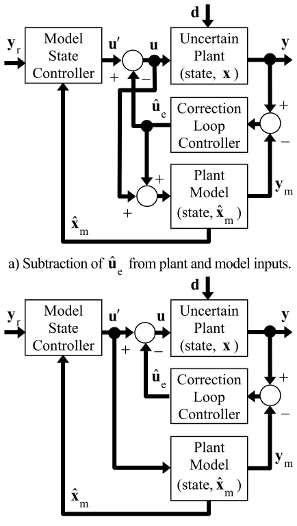
Fig. 2.3: Structure of OBRC.

Since the plant model must be mismatched with respect to the real plant, the well known separation theorem of control system design doesn’t strictly apply and to prove closed loop stability, the system as a whole would have to be analysed. Intuitively, however, the measurement vector, y, can be regarded as a disturbance input to the observer correction loop that is ‘rejected’ by being counteracted by y_m if the correction loop gains are sufficiently high and determined using only the plant model. This has been confirmed by many simulations and some experiments currently

needed from an academic viewpoint.

The control system is completed by forming the primary control input according to (2.6), followed by loop closure around the model using a state feedback controller to generate the primary control input, as shown in Fig. 2.3 (a). After simplification of the input connections, Fig. 2.3 (b) shows that the subtraction of uˆ_e from the plant and model causes only u′ to be applied to the plant model and the correction loop controller to be applied to the plant. Remarkably, this proves to be a method of applying a high gain loop to an unknown plant while ensuring stability.

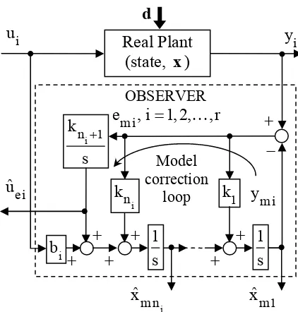
2.3. Choice of observer plant model. In cases where a linear plant model is readily available, then it is recommended that this is used as a basis for the controller design. If not, however, modelling can be the most time consuming and therefore costly activity required to produce a control system design. OBRC can avoid this and provide robustness since, remarkably, there is no requirement for the plant model to closely resemble the real plant for equation (2.5) to be readily soluble. With this freedom, the plant model is chosen as chains of integrators separately driven by each control input. Not only will this yield straightforward design of the two controllers in Fig. 2.3 but for multivariable plants, ensure elimination of closed loop interaction between control channels. The observer then comprises r separate single input, single output sub-observers as shown in Fig. 2.4.

− +

Uncertain Plant (state, x)

Plant Model (state,xˆ_m)

u

+

y

Correction Loop Controller

+

−

e

ˆ

u

+ ′

u

m ˆ x

Model State Controller r

y

m y

a) Subtraction of uˆ_e from plant and model inputs.

−

u

e

ˆ

u

+

Uncertain Plant (state, x)

Plant Model (state,xˆ_m)

d

y

Correction Loop Controller

+

− ′

u

m ˆ x

Model State Controller r

y

m y

Fig. 2.4: Multiple integrator based observer. Although it would make no difference to the response of the ideal system in which

mi

e =0 the integrator chain gain, b , is _i included as an adjustable parameter because with finite observer gains it would affect the accuracy of ˆu . _ei

Finally but importantly, if the total number of integrators in the chains is less than the plant order and the plant is of full rank, i.e., the sums of the relative degrees with respect to each output is equal to the plant order, then the order of the closed-loop system would be less than the plant order, resulting in closed-loop modes, unobservable by viewing the reference inputs and outputs, that could be unstable. This could be avoided by making the total number of integrators exceed the plant order but for plants not of full rank, there would be zero dynamics of the closed loop system unobservable in the aforementioned sense similar to that experienced in sliding mode control (Utkin, 1992). This would also enable the controller to accommodate a range of plants of different orders in a similar fashion to hyper-sliding mode

control (Dodds, 2006) while yielding the same closed loop dynamics.

A method commonly included in state controllers for electric drives (Vittek and Dodds, 2003) to estimate external disturbances is to add an integrator to the observer model, as exemplified by the additional integrator with gain,

i n 1

k ₊ , in Fig. 2.4. In view of the OBRC theory presented in section 2.2, this also includes the effects of the mismatched between the plant and its model so the output of this integrator can be taken as ˆu . Inclusion of _ei this integrator also ensures zero steady-state error between y_r and y due to constant components of d. The model correction loop of Fig. 2.4, however, is not of the same form as that of Fig. 2.2, several different correction paths being implemented instead of one. Fig 2.4, however, could be converted to the same form with a single correction loop controller. This would entail adding derivative terms to the ‘

i n 1

k ₊ ’ integrator output but since the observer of Fig. 2.4 is sufficient to estimate u_e, using the precise observer structure of Fig. 2.2 will be left to a future investigation.

3. Speed and position control of a

synchronous motor drive.

3.1 Modelling and OBRC formulation. The permanent magnet synchronous motor (PMSM) is modelled in the synchronously rotating d-q co-ordinate system by the following set of state differential equations:

di_d dt= −Ai_d+ ωB i_{r q}+Fu_d (3.1)

di_q dt= − ωC i_{r d}−Di_q− ω +E _r Gu_q (3.2)

i m n

ˆx ˆx_m1

ei ˆu

− +

+ +

+

i u

+

i n 1 k

s

+

Real Plant (state, x)

d

i y

mi y mi

e , i 1,2, ,r= _K

1 s 1

s

1 k

i n

k

+ +

Model correction

loop

i b

r d q L

r r

dϑ dt= ω (3.4)

where i_d, i and _q u_d, u are the stator _q

current and voltage components, ω_r is the rotor angular velocity and Γ_L is the external load torque (Vittek & Dodds, 2003). Here:

( )

(

)

( )

(

)

s d d

q d q

d q PM r

s q d q r

PM q r L

A R L ; F 1 L

B p L L ; G 1 L

C p L L ; H 3p 2J

D R L ; K 3p L L 2J

E p L ; M 1 J J

= =

 

= =

 

 _{= = Ψ}

 

= = −

 

= Ψ = +



PM

Ψ is the permanent magnet flux, R_s is the stator resistance, L_d and _Lq are the direct and quadrature axis inductances, J _r and J are the rotor and load moments of _L inertia and p is the number of pole pairs. For position and speed control, the controlled measurement variables will be, respectively:

1 r

y = ϑ (3.5) y₂ = ω_r (3.6) These measurements are derived from shaft encoder outputs and are scaled to be numerically equal to the physical quantities being measured. There will be an additional controlled measurement variable:

3 I d

y =K i (3.7)

since this has to be controlled with y_3r =0 to maintain the flux and current vectors mutually perpendicular for maximum torque generation efficiency (vector control). It is clear from (3.1) and (3.7) that the relative degree is 1 w.r.t. y₃, because the control variable, u_d, already appears on the RHS of

lower integrator chain of Fig. 2.4. For the speed control, differentiating (3.6) twice and substituting for di_q dt using (3.2) yields the

other control variable, u , on the right hand _q

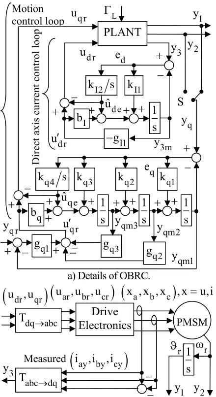
side and therefore the rank is 2 w.r.t. y . It is ₂ 3 w.r.t. y due to the kinematic integrator in ₁ (3.4) and this would require three integrators in the lower chain of Fig. 2.4. The same controller will be used for y as the number ₂ of integrators in the chain exceeds the plant rank w.r.t. this output by 1, which is acceptable. Fig. 3.1 shows a block diagram of the complete observer based robust control system (switch S to y or ₂ y ). The ₁ subscripts, r and y, refer, respectively to reference inputs and measurements and the transformations are as follows, with intermediate stator-fixed α-β frame:

Park Transformation

Clark transformation dq

3

abc

abc dq

i

2 1 1 _ay

i_{dy cos sin 3 3 3}

i_by

i_qy sin cos ₀ 1 1

i

3 3 _cy

T y

T i_dy

T

αβ→

→αβ →

 

 _{− −} 

  _{ θ θ}  

 _{=  }  

− θ θ

    ₋  

  _{  }

 _{  }

=

1442443

1442443

144444424444443

(3.8)

Inverse Park Transformation Inverse Clark _dq Transformation

abc

dq abc

1 0

u_{ar u}

cosθ sinθ

1 3 _dr

u_{br u}

sinθ cosθ

2 2 _qr

u_cr

1 3

2 2

T

T

T

→αβ

αβ→

→

 

 _{  }

 

  _{ } − 

= −  

  _{  }

 

 

  _{   }

 

 _{  }

− −

 

 

1442443

1442443

1444442444443

Fig. 3.1: OBRC applied to electric drive for position or speed control.

Figure 3.2 shows a block diagram of the motor based on the two-phase model (3.1) to (3.4) with transformations (3.8) and (3.9) for the three-phase stator voltages and currents. Since the real time models are chosen as integrator chains, design by pole placement is very straightforward and mathematically similar for the observers and model state controllers. Applying the author’s settling time formula (Vittek and

Dodds, 2003) the characteristic polynomial for n coincident

Fig. 3.2: Model of motor with transformations for three-phase stator

voltages and currents.

poles and a settling time, T_s, is given by:

( ) n

s

s 1.5 1 n T

 + + 

  (3.10)

Applying this with the appropriate values of n and the specified settling times, T_soI,

scI

T , T_soq and T_scq of the observer correction loops and then equating with these characteristic polynomials obtained from Fig. 3.1 (a) using Mason’s formula, yields:

2 2

I1 I2 2

soI _soI

9 81

s k s k s s

T _4T

+ + = + +

4 3 2

q1 q2 q3 q4

2 3

4 3 2

2 3 4

soq _{soq soq soq}

s k s k s k s k

4a 6a 4a 1 15

s s s s , a

T _{T T T} 2

+ + + + =

+ + + + =

I1 scI

s g+ = +s 3 T

3 2

q3 q2 q1

3 2

2 3

scq _{scq scq}

s g s g s g

18 108 216

s s s

T _{T T}

+ + + = + + + − qm3 y + d r u′ + − + 3m y qe

ˆu ₊

2 y r ω r ϑ −

(

)

2 y 1 y 3

y Measured

(

)

− d e + + q r u′ de ˆu ₊

− + + + + 3 y + d r u PLANT L Γ 1 y q r u − 1 s I1 k I2 k s − I1 g − qm2 y + − 1 s q1 k q4 k s q1 g S 1 s q2 k q2 g q y q r y qm1 y +

Direct axis cu

rrent control l

oop abc dq T _→ dq abc T _→ q e Drive

Electronics PMSM

(

)

(

)

1 s

b) Plant: drive electronics and measurement blocks, with 2/3 and 3/2 phase transformations.

a) Details of OBRC.

+ _{1 +}

s q3 k q3 g I b q b Motion control loop 1 y − − − + + + + + + q i r ω 1 s 1

s A+ F

1 s D+

in s then yields to following gain equations:

I1 I2 2 I1

soI _soI scI

9 81 3

k , k , g

T _4T T

= = = (3.11a)

2 2

q1 soq q2 soq

3 3 4 4

q3 soq q4 soq

k 4a T ,k 6a T ₁₅

a 2

k 4a T ,k a T



= =

 = 

= = _ (3.11b)

q3 q2 2 q1 3

scq _{scq scq}

18 108 216

g , g , g

T _{T T}

= = = (3.11c)

3.2. Simulations

The PMSM parameters are as follows: 2

r

J =0.003 Kgm ; p 3= ; L_d =1.4 H;

q

L =0.1618 H;

s

R =36.5; Ψ_PM=0.312 Wb.

The mechanical load moment of inertia is 2

L

J =0.01 Kgm . The current transducer gain is K_I =0.5V / A. The position and velocity measurements are assumed to obtained from a shaft encoder and scaled to be numerically in rad/s and radians, so

K_ω=K_ϑ =1.

The effects of a power electronic drive with a 300V d.c. link voltage with a switching frequency of 20 kHz is simulated by applying corresponding square wave perturbations to u to obtain _ir u , _i

i a,b,c= .

The OBRC parameters are set to

scI scq

T =T =0.2s and T_soI =T_soq =0.05s. All the simulations start with zero initial conditions. For speed control, the step reference angular velocity is y_2r =K_ωω_{r r} where ω =_{r r} 200 rad / s and for position control, the step reference angle is

robustness against external disturbances is assessed by applying an external load torque, Γ_L( )t , at t 0.5s= that ramps at 100 Nm / s to a constant value of 3 Nm. The integrator chain gains are b 1_I= ;

q

b =600.

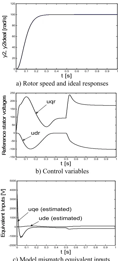
Fig. 3.3 and Fig. 3.4 show the speed and position control responses.

0 0.1 0.2 0.3 0.4 0.5 0.6 0.7 0.8 0.9 1 0

20 40 60 80 100 120

t [s]

y2

, y

2i

d

e

al

[r

ad

/s

]

a) Rotor speed and ideal responses

0 0.1 0.2 0.3 0.4 0.5 0.6 0.7 0.8 0.9 1 -150

-100 -50 0 50 100 150 200 250

t [s]

R

ef

er

enc

e s

ta

tor

v

ol

tages

udr uqr

b) Control variables

0 0.1 0.2 0.3 0.4 0.5 0.6 0.7 0.8 0.9 1 -2000

-1000 0 1000 2000 3000 4000 5000

t [s]

E

q

ui

va

le

nt

I

npu

ts

[

V

]

ude (estimated) uqe (estimated)

4. Conclusions and recommendations

Despite the plants simulated being different, even in order, the response shapes are identical and indistinguishable from the ideal responses and the errors due to the load torque are invisible on the scales of the reference inputs. The control variables needed are, of course, very different. The model mismatch equivalent input for the q-axis exceeds the supply voltage but this is not problematic because it is only an internal

0 0.1 0.2 0.3 0.4 0.5 0.6 0.7 0.8 0.9 1 0

0.5 1 1.5 2 2.5

t [s]

y1

, y

1i

deal

[

rad]

a) Rotor angle and ideal responses

0 0.1 0.2 0.3 0.4 0.5 0.6 0.7 0.8 0.9 1 -100

-50 0 50 100 150

t [s]

Ref

e

re

nc

e S

tat

o

r V

o

lta

ge

s

uqr uqr

udr

b) Control variables. Fig. 3.4: Position control.

variable in the control computer, the physical control inputs staying within a practicable limits of 400V± .

OBRC is a promising new control method but theoretical work must be done regarding stability limits in view of the

need to employ finite observer gains in practice.

5. References

Yamada, K., ‘Modified Internal Model Control for Unstable Systems’, Proceedings of MED99, Haifa, Israel, June 28-30, 1999.

Utkin, V. I., Sliding Modes in Control and Optimisation, Springer Verlag, 1992.

Dodds, S. J., “Hyper Sliding Mode Control”, Proceedings of AC&T 2006.