Sounding response calculation of layered model surface based on nuclear magnetic resonance

Journal of Chemical and Pharmaceutical Research, 2014, 6(5):324-332

Research Article

_{CODEN(USA) : JCPRC5}

ISSN : 0975-7384

Sounding response calculation of layered model surface based on

nuclear magnetic resonance

1

Chu Yan,

1

Cai Xin-yuan,

2

Bian Dong-yan,

1

Sun Nai-hua and

1

Tang Kang

1

Electronic & Control Engineering Department, Chang’an University, Xi’an, China

2

Senior Technical University of Puyang, Puyang, China

____________________________________________________________________________________________

ABSTRACT

At present, the calculation of nuclear magnetic resonance sounding simulation is mainly based on homogeneous half space model or equivalent half space model. As the equivalent model makes the calculation result vary greatly from the actual response, in order to avoid the error brought by the equivalent model, the paper first implement the oscillating integral calculation by using gauss numerical integration and gets the scattering field of the underground space based on layered model harmonic field electromagnetic response derived by the recursive method, then obtains nuclear magnetic resonance (NMR) sounding response under one-dimensional medium case. In order to verify the effectiveness of the proposed algorithm, the layered model of calculation method is used to calculate the homogeneous half space of NMR response, being consistent with the actual uniform half-space model results, indicating that the calculation method given in the text reliable. The paper calculated the different orientation of the cutting angle under toppled layered model, and compared the differences in cross-sectional direction of cutting angle. Analysis is showed that NMR response is calculated more accurately by layered model recursive method than by the method of approximate half-space model.

Key words: Layered model; electromagnetic response; NMR; scattering field

____________________________________________________________________________________________

INTRODUCTION

MAGNETIC FIELD DISTRIBUTION OF LAYERED MEDIUM Theoretical expression of magnetic field in layered media

Under the circular loops conditions, the horizontal component Hr and vertical component Hz of any point in layered medium ground can be written as[3,4,5,6,7]:

(1)

0 (1) 1 0

0 0

(

)

(

)

z

z

H

I a

J

a J

r d

z

z

λ

_λ

_λ

_λ

∞

=

+

∫

(1)

In the first layer, the electromagnetic field is expressed as:

1 1

1 1 1 1 1 1

0

(

) (

)

2

u z u z

r

Ia

H

a e

b e

u J

λ

a J

λ

r d

λ

∞ −





=

_∫

_

+

_

(2)

1 1

1 1 1 1 0 2

0

(

)

(

)

2

u z u z

z

Ia

H

a e

b e

λ λ

J

a J

λ

r d if

λ

∞ −





=

_∫

_

+

_

(3)

Where

a

₁,

b

₁is undetermined coefficients,

I

is emission current,

a

is the radius of the transmitter block,

r

is

the offset distance,

z

is the depth,

u

_i

=

λ

2

−

iw u

σ

_{i 0} ,

w

is the frequency of the emission current,

σ

_iis the

electric conductivity in the

i

-layer,

u

₀ is the vacuum permeability.

According to the boundary conditions of horizontal component being equal to a vertical component at the interface of the magnetic field, it can be obtained:

1 1

(2) (1)

2 1

1 (1) (2)

0 1

2

(1

z

z

u h

)

z

a

e

z

z

z

z

−

−

=

+

+

+

(4)

1 1

(2)

2 1

1 (2) 1

1

u h

z

z

b

e

a

z

z

−

−

=

+

(5)

Where,

h

_i is the total thickness of the former

i

layer, where

z

( )i and

z

i have the following recurrence relations:

i i i

i u

z

u

ω

−

=

(6)

( )1

( )

( 1)

(

)

(

)

i

i i i i

i i

i i i

z

z th u H

z

z

z

z

th u H

+ +

+

=

+

(7)

In the lowermost layer:

( )n n

z

=

z

(8)

In the

i

-layer medium, undetermined coefficients

a

_i,

b

_i satisfy the following relationship:

( 1) ( 1) i i i iu h i

i i i

i

z

z

b

e

a

z

z

+ − +

−

=

+

(9)

First step is to obtain first layer magnetic field expressions undetermined coefficients, then the field values on the first layer to the interface can be obtained after coefficients substituted into the expression, based on the relationship between the field continuity and the second magnetic layer undetermined coefficients, finally

a

₁,

b

₁ in second layer can be obtained, so undetermined coefficients in each layer can be calculated.

Calculation of the magnetic field in layered media

double infinite integral Bessel functions [8,9]. The integral in the problem is no analytical expression, so only the numerical method is used for solving integral. In order to ensure the accuracy and precision of the integral, the form of integral function must be figured out before integral, uniform half-space vertical magnetic field is expressed as:

1

2

0 1 0

0

(

)

(

)

u z

z

i

H

I a

J

a J

r e

d

u

λ

_λ

_λ

_λ

λ

∞

−

=

+

∫

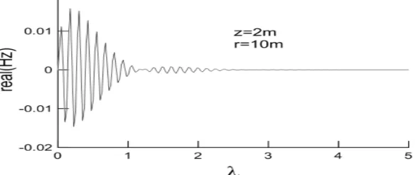
(10)

[image:3.595.163.457.198.321.2]

Integrand values in the vertical magnetic field expression (10) change with the independent variables shown in Figure 1.

[image:3.595.163.451.345.464.2]

Fig. 1: The function value variation regulation of the vertical magnetic field integrand real part

Fig. 2: The function value variation regulation of the vertical magnetic field integrand imaginary part

The oscillation of the vertical magnetic field plot function’s real part is very strong, and imaginary part is small, in order to ensure the accuracy of integration, the plot function properly be handled before integration. The vertical component of the magnetic field is written as follows:

1 2 3

zi

H

= + +

f

f

f

(11)

Where

1 1

(

)

0

(

)

2

j j

u z u z z

j j

Ia

f

=

∫

λ



_

a e

−

+

b e

−

e

−λ

_



J

λ

a J

λ

r d

λ

(12)

[

]

2 1 0

0

(

)

(

) 1

2

z

Ia

f

λ

e J

λ

λ

a J

λ

r

d

λ

∞

=

_∫

−

(13)

3 1

0

(

)

2

z

Ia

f

λ

e

λ

J

λ

a d

λ

∞ −

=

_∫

(14)

1

f

is the value that the vertical variable

H

_zsubtracted the value generated by transmitter loop in the air, the

[image:4.595.166.450.63.206.2]

Fig. 3: The function value variation regulation the real part of

f

₁integrand

After processing, the plot function will quickly decay to zero, and the oscillation disappears, the integration interval can be defined as [0, 1] to ensure the integration accuracy.

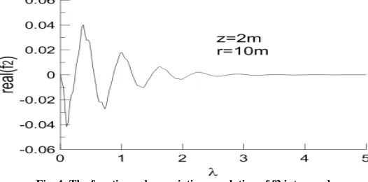
Because of the double Bessel function aggravating the shock of integral function, the shock of a Bessel function fairly to double Bessel function after performing minus 1 to a Bessel function

f

₂, the relationship between

[image:4.595.175.438.320.450.2]

the

f

₂of integral function and the independent variables is shown in Figure 4.

Fig. 4: The function value variation regulation of f2 integrand

Since

f

₂expression contains an exponential decay term, the integration interval is limited, it can be set to [0, z],

z

is the depth of the point, Gaussian integral is performed in each elements section by the subdivision of integration interval, the value of the integral can be obtained, and

f

₃ is a special analytic integration, the result is:

2

3 1 3

2 2

0 2

(

)

2

2(

)

z

Ia

Ia

f

e

J

a d

a

z

λ

λ

λ

λ

∞ −

=

=

+

∫

(15)

Through the first two steps of processing, the integral contained Bessel function is changed into the total of double and three, and each of the integral is easy to implement [10,11,12].

The calculation of the actual model magnetic field distribution

In order to determine the calculation of initial NMR amplitude’s grid mesh spacing and range, spatial distribution of the magnetic field under different model parameters is calculated. Each model parameters is shown in Table 1.

Table.1 Geoelectrical model in Fig 1and Fig 2

Model ρ1/Ω·m h1/m ρ2/Ω·m h2/m ρ3/Ω·m

1 100 30 100 20 100 2 100 30 30 20 100 3 100 30 5 20 100

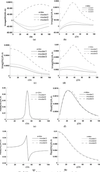
the perpendicular magnetic field is largest in the radius of the coil, but the reverse direction does not occur which is consistent with the law of the magnetic field lines being closed to near energized wires. The middle layer resistivity change affects little to the real part of the magnetic field of cover layer, instead of the imaginary part changing with the resistivity a lot. The value of the imaginary part of the magnetic field is smaller than the real part. For a radius of 50 m emission circular loop, whether horizontal or vertical component of the magnetic field component, when the offset distance is greater than 100 m, the values is close to 0.

(a) (b)

(c) (d)

(e) (f)

[image:5.595.140.474.150.720.2]

(g) (h)

Fig. 5: Magnetic field components variation in covering layer

(a) Hr imaginary part variation along radius (b) Hr imaginary part variation along depth (c) Hz imaginary part variation along radius (d) Hz imaginary part variation along depth (e) Hr real part variation along radius (f) Hr real part variation along depth (g) Hz real part variation

The distribution of the magnetic field in aquifer directly determines the distribution of proton magnetic moment toppled angular under the same pulse major, each figure of figure 6 (a)-(d) reflect the change rule long radial of magnetic field real and imaginary parts in low resistance sandwich. When the low-resistivity layer exists, the imaginary part of the magnetic field is affected greatly in the upper medium, with the decrease of the resistivity of the low resistance sandwich, whether the imaginary part of the vertical component or the horizontal component will change a lot, but little effect to the real part. In the low-resistivity layer, with sandwich lower resistivity, the greater the difference exists in the imaginary part of each component of the magnetic field, and the real part begin to change a little. Only when the low resistivity is down to 10

Ω

, this difference will behave out. The vertical component of the deep magnetic field has no changes in the radial direction compared with shallow the magnetic field, but with the increase of an offset distance, the value of the magnetic field decreases, the horizontal component of the magnetic field is still the maximum radius of the coil. However, when the mutations disappear, the horizontal component varies slowly component along the radial. In order to verify the correctness of the calculation result, the magnetic field at the center of the uniformity earth loop is calculated. According to the analysis result, when the resistivity was 100

Ω

, loop radius 50m, the emission current 1 A, the frequency 2350

Hz

, the size of central vertical magnetic field loop is (9.832e-3,1.657e-4), and the results obtained by numerical integration methods is (9.958e-3,1.816e-4) with very small error, the results show that the calculation is credible.

(a) (b)

(b) (d)

Fig. 6: Magnetic field components variation in low resistivity layer

(a) Hr imaginary part variation along radius (b) Hz imaginary part variation along radius (c) Hr real part variation along radius (d) Hz real part variation along radius

THE CALBULATION OF SURFACE NMR RESPONSE

Under the excitation of the surface feeding Larmor frequency sinusoidal current and electromagnetic waves, the direction of proton magnetization will deviate from the direction of the geomagnetic field. As time increases, the angle of deviation increases. when the excitation stops, the direction of protons magnetization will gradually coincide with the direction of the geomagnetic field [13,14]. In this process, the signal decaying with time in surface coil can be observed, the theoretical attenuation of the signal is calculated as (16).

2

0 0

( , )

( )

cos(

)

t T

E Q t

E Q e

wt

ϕ

−

=

+

(16)

Where,

Q

=

It

_pis the product of the excitation current intensity and the duration time, E is the initial amplitude of

the

Q

pulse moment,

t

₂is transverse relaxation time,

w

is the Larmor frequency,

γ

is the proton gyromagnetic

0

0

( )

sin(

) ( , , )

wM

E Q

B

B t n r

z dv

I

⊥

γ

⊥

ϕ

=

_∫∫∫

(17)

0

M

is the size of the proton magnetization,

B

_⊥ is component of the excitation magnetic field strength perpendicular to the field. In the case of the cylindrical coordinate,

n r

( , , )

ϕ

z

is moisture content the point of

( , , )

r

ϕ

z

.

NMR signal is the result of the volume integrals to the underground aquifer, the degrees of motivation is different in different locations. This difference reflected in the different spatial positions is toppled the corner. The size of aquifer toppled angle directly affects the size of the size of the NMR signal. The angle toppled sandwich in three sectional distribution of models 3 is calculated where the angle between the profile and the plane of the earth's

magnetic field is respectively

0

o,

45

o,

90

o, geomagnetic inclination is

60

o, excitation pulses is

1A s

⋅

. The result is shown in figure 7:

(a) (b)

(c)

Fig. 7: Toppled angle distribution in different profile

(a) South-north direction profile (0 degree) (b) North-east direction profile (4degree) (c) East-west direction profile (90 degree)

In the different directions of cross section, toppled angles distributes differently. In the

0

o cross-section, the distribution of the toppled angular is asymmetry and the toppled angular distribution is scale in the cross section of

90

o, but the value of toppled angle is the minimum.

0

0 ( , , ) ( , , )

1 1 1

( )

sin(

)

M N K

m n k m n k

m n k

wM

E Q

B

B

t dv

I

= = = ⊥

γ

⊥

=

∑∑∑

(18)

Since the medium is assumed layered,

r

and

ϕ

can be the first integration, and then the z integrating, the integration interval is split a summation of discrete points according to the column:

m m n k

r

∆

，

∆

φ

，

∆

z

are respectively the radial，tangential directions and the split in length depth, the size of

subdivision length can be determined according to accuracy requirements, combined with the literature and the

results, the integration interval can be set to

x

2

+

y

2

≤

4

R z

2

,

≤

2

R

,with transmit coil radius of

R

, outside this range, the value of the magnetic field is small, the impact on the calculation results is insignificant.

Taking the rapid change of magnetic field near the coil into account, while slow changes happens in other places, the spacing may be unequal subdivision according to the distribution of magnetic field mesh. Coupling the variation of magnetic field in the vertical and horizontal direction and in the radial direction, mesh spacing of 0-40m is 2m, mesh spacing of 40-60m is 1m, mesh spacing of 60-100 is 2m. It is evenly split the direction of

φ

, the circle is divided into 36 parts uniform domain, using a uniform mesh spacing of 2m in the

z

-direction.

[image:8.595.173.445.302.561.2]

Make a numerical calculation for the three layer model, the resistivity of the first, the third layer are 100

Ω⋅

m

, the resistance of the intermediate layer respectively is 100,30,10,5

Ω⋅

m

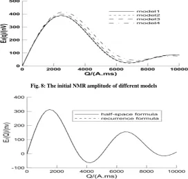
. The first and the second floor thickness is respectively 30m, 20m assuming low resistance caused by water, and the interlayer low resistance is representative of the aqueous layer, thickness of the interlayer is depth of water. When the transmitter loop radius is 50m, the water content is 10%, the emission current is 1

A

.The variation of initial pulse amplitude is shown in figure8 and figure 9 when resonant frequency is 2350

Hz

:

Fig. 8: The initial NMR amplitude of different models

Fig. 9: The initial NMR amplitude of different algorithm

Figure 9 shows the results of the using a uniform half-space formula and recursive formula to calculate NMR initial amplitude of uniform half-space, model resistivity is100

Ω⋅

m

, aquifer thickness is 10m, depth is 20m, the water content is 10%.There is no difference between the two methods of calculation results proving the reliability of the recursive method.

CONCLUSION

(1) NMR forward simulation is to solve the problem of the double Bessel function integral. Integration interval is greatly reduced by subtracting magnetic field generated by transmitter coil in the air. The oscillation will reduce by doing one minus processing to Besesl function and make the calculation of the magnetic field become feasible.

(2) The impact resistance of the magnetic field is mainly reflected in the imaginary part of the magnetic field, the high resistance layer, the difference of the imaginary part is relatively small, however, in the low-resistivity layer, the difference is very obvious. The real part of the magnetic field is sensitive to changes of resistivity, this effect is

(3) For layered media, the magnetic field can be directly calculated using recursive methods, without the need of an equivalent model which avoid bias caused by equivalent model and improve the accuracy of the calculation results.

Acknowledgements:

The authors would like to thank the coverage area of mineral resources prediction and results summary for support under the grants (1212011085468).

REFERENCES

[1] Anatoly Legchenko,Jean-Michel Baltassat,Alain Beauce. Journal of Applied Geophysics, 50:21～46,2002.

[2] Kamhaeng Wattanasen, Sten-Ake Elming. Journal of Applied Geophysics, 66:104～117,2008.

[3] WENG A H,LI Z B, Wang X Q. Computing techniques for geophysical and geochemical exploration.(in

Chinese), 24(2):97～98,2002.

[4] WENG A H,LI Z B, Wang X Q. Chinese Journal of Geophysics.(in Chinese ), 47(1):156～158,2004.

[5] LI Xing. Shanxi scientific and Technological Press, 35(1):124~131,2002. [6] QI Z P. Master Thesis of Chang’an University,23(2):347~354,2008.

[7] XUE G Q,LI X,GUO W B,DI Q Y. Geophysics for oil exploration.(in Chinese), 42(5):586～590, 2007.

[8] HUA J,JIANG Y S,WANG W B. Coal geology and exploration.(in Chinese),29(03):58～61, 2001.

[9] ZHANG W,WANG X B,QING Q Y. Geophysics and Geochemical exploration.(in Chinese),12,34(6):753～755,

2010.

[10] ZHANG H,LI T L,DONG R X,XU K J. Progress in Geophysics.(in chinese), 2005.9,20(3):667～670.

[11] WENG A H,WANG X Q. Northwestern seismological Journal.(in Chinese) ,25(3):193～197, 2003.

[12] A.Legchenko, M.Ezersky, J-F.Girard etal. Journal of Applied Geophysics. 66:118～127,2008.

[13] C.L. Bray, N.C. Schaller, S.L. Iannopollo, M.D. Bostick. Journal of Environmental and Engineering

Geophysics.11(1):2, 2006.