Analysis of partial least squares algorithm based on SBM DEA

Journal of Chemical and Pharmaceutical Research, 2014, 6(7):718-724

Research Article

_{CODEN(USA) : JCPRC5}

ISSN : 0975-7384

Analysis of partial least squares algorithm based on SBM-DEA

Jianqiang Du

1

, Zhulin Hao

1

, Guolong Wang

1

, Riyue Yu

2

, Bin Nie

1*

and Wangping Xiong

1

1

School of Computer, Jiangxi University of Traditional Chinese Medicine, Nanchang, China

2

School of Pharmacy, Jiangxi University of Traditional Chinese Medicine, Nanchang, China

_____________________________________________________________________________________________

ABSTRACT

The

T

2ellipse assisted analysis method of the partial least squares (PLS) is able to recognize the noise, however, it fails to analyze the noise in the multidimensional space. In the paper, we propose the slacks-based measure ( SBM ) algorithm to optimize PLS. Firstly, evaluating the sample data comprehensively with SBM, we can gain the valid data. Secondly, analyzing the data based on the PLSR. The two steps can avoid the impact which the noise data have on the regression accuracy and make up the aided analysis technology of the PLSR. Through the calculation of traditional Chinese medicine (TCM) experiments, for two dependent variables, we find out that the average relative errors of the optimized PLS with SBM algorithm are 5.0844% and 8.7485%, which are lower than the results ( 5.5825% and 9.2810% ) by using the PLSR. Besides, for a single dependent variable of the data of tool wear test, the average relative error optimized by SBM is 2.6984%, which is lower than 3.3526% calculated by utilizing the PLS. The experiments result indicate that the regression precision of the PLSR optimized by SBM is much higher than PLSR.

Key words: DEA; slacks-based measure; PLS; auxiliary analysis technology

_____________________________________________________________________________________________

INTRODUCTION

THE SBM-DEA ALGORITHM

Data envelopment analysis put forward by Charnes A[6] can be used to estimate the relative efficiency of the decision making unit with multiple inputs and multiple outputs. The traditional DEA (such as CCR and BCC) ensures the boundary of the relative effectiveness or the convex of the indifferent curve, but it may lead to the congestion and slacks of the inputs[7]. It is more difficult for all the each decision making unit the overall data samples to evaluate the relative effectiveness, when increasing the input or output and considering the corresponding slack. Kaoru proposes SBM[8] of efficiency in Data Envelopment Analysis. This scalar measure deals directly with the output shortfalls and the input excesses of the decision making unit (DMU) concerned, so it is a effective method to solve the slacks issue[9].

We will dispose

n

DMUs with

s

₂ undesirable outputs,

s

₁ good outputs and

m

input matrices, 2

(

)

m s b

ij

Y

=

y

∈

R

× , g

₍

₎

m s1

ij

Y

=

y

∈

R

× and

X

=

( )

x

_ij

∈

R

m n× . Suppose that the data samples are positive, i.e.

0

X

>

and

Y

>

0

.Hence, SBM model is shown by the following:

1 2

1 0

1 1

1 2 0 0

0 0 0

1

1

min

1

1

.

0,

0,

0,

0

m

i i i

s g s u

i r

g b

r r r r

g g g

b b b

g b

s

m

x

s

s

s

s

y

y

X

s

x

Y

s

y

s t

Y

s

y

s

s

s

ρ

λ

λ

λ

λ

− = = = − −

−

=





+



+



+







_{+ =}



−

=





+ =





_≥

_≥

_≥

_≥



∑

∑

∑

(1)

where

ρ

is an effort to estimate the efficiency, the vectors

s

−

∈

R

m、

_s

g

∈

_R

s1_and

_s

b

∈

_R

s2 _{indicate the input} excess and output shortfall in this expression, respectively, and are called slacks.For the particular decision making unit evaluated as follows:

Definition 1:

(1) A DMU is SBM-efficient if

ρ

=1

which is equipment to

s

g

=

0

,

s

b

=

0

and

s

−

=

0

;

(2) A DMU is weak effective but close to the effective, existing the necessity of the input and output improvement.The problem given above is a nonlinear programing because of containing the nonlinear term. To facilitate the use of MATLAB programing calculation, utilizing the Cooper transformation[10], we can transform it into a linear program as follows:

1 2

1 0

1 1

1 2 0 0

* 0 * 0 * 0 *

1

min

1

1

.

0,

0,

0,

0,

0

m i i i b

s g s

i r

g b

r r r r

g g g

b b b

g b

S

t

m

x

S

S

t

s

s

y

y

X

S

x t

s t

Y

S

y t

Y

S

y t

S

S

S

t

ρ

λ

λ

λ

λ

− ∗ = = = − −

=

−







+

+

=







+









₊

₌





−

=





₊

₌



≥

≥

≥

≥

≥



∑

∑

∑

(2) * *

,

t s

,

S

t s

,

g

S

g

t s

,

b

S t

b

ρ ρ λ λ

₌

₌

−

₌

−

₌

₌

A NOVEL APPROACH BASED ON SBM-DEA

(1) Suppose that

S

=

( ,

s s

_{1 2}

,

L

,

s

_m

)

is the data samples,

m

is the number of samples, independent variables and dependent variables are

( ,

x x

_{1 2}

,

L

,

x

p

)

and

( ,

y y

1 2

,

L

,

y

q

)

. According to the SBM model,

1 2

( ,

s s

,

L

,

s

_m

)

is took as decision making unit, called stations of the data samples;

( ,

y y

_{1 2}

,

L

,

y

_r

)

is the undesirable outputs not being expected to increase;

(

y

r+₁

,

y

r+₂

,

L

,

y

q

)

is the good output being expected to

increase;

( ,

x x

_{1 2}

,

L

,

x

_p

)

is the input. Then, (2) is adopted to solve

ρ

of the decision making unit. For a sample, we call the sample as the effective sample if

ρ

=

1

, namely, the effective value of the SBM model take the threshold for 1 as a standard. Therefore, the new selected data samples are analyzed by utilizing partial least squares method. The concrete SBM algorithm workflow is as follows:

Input :

S

=

( ,

s s

_{1 2}

,

_L

,

s

_m

)

Output :

ρ

Initialize : Repeat

Compute

ρ

Using the formulation (2) Until converge

Result :

* *

,

t s

,

S

t s

,

g

S

g

t s

,

b

S t

b

ρ ρ λ λ

₌

₌

−

₌

−

₌

₌

(2) The effective data sample selected through step(1) is preprocessed. Then we get the processing data matrix: The independent variables are

X

=

( ,

x

₁

L

, ,

x

i

L

,

x

p

)

; The dependent variables are

Y

=

( ,

y

1

L

,

y

j

,

L

,

y

q

)

, where

n

is the number of the data samples,

p

is the number of the independent variables,

q

is the number of the dependent variables.

(3) Let

t

₁ and

u

₁ be the first principal component of

X

and

Y

,i.e.

t

₁

=

Xw

₁,

u

₁

=

Yv

₁, where

w

₁ and

v

₁ are the first axis of

X

and

Y

, i.e.

v

₁

=1

,

w

₁

=1

,these axises are the unit column vector.

t

₁ and

u

₁ must meet the following two conditions[12]:

1) the variation information is the largest:

Var t

( )

₁

→

max,

Var u

( )

₁

→

max

2) the degree of correlation is the biggest too:

r t u

( ,

_{1 1}

)

→

max

It can get that the covariance is the maximum synthetically:

Cov t u

( ,

_{1 1}

)

=

r t u

( ,

_{1 1}

)

Var t Var u

( )

₁

( )

₁

→

max

Then basing on the Lagrange Algorithm, we can obatain:

X

=

t p

_{1 1}T

+

X

₁ 1 1 1

T

Y

=

t r

+

Y

where

X

₁ and

Y

₁ are the residuals information matrix of

X

and

Y

, the regression coefficient vector

p

₁ and

1

r

are as follows:

1

1 2

1

1

1 2

1

T

T

X t

p

t

Y t

r

t



=









₌





(3)

1 2

2 2

2

1 2

2 2

2

T

T

X t

p

t

Y t

r

t



=









₌





(4)

(5)So we recycle residuals information matrix to calculate iteratively, and assume the rank of

X

to be

m

(if it has

A

principal component,

A

≤

r X

( )=

m

),then it has:

1 1 2 2

1 1 2 2

+

T T T

m m m

T T T

m m m

X

t p

t p

t p

X

Y

t r

t r

t r

Y



₌

₊

_{+ +}

₊





=

+

+ +



L

L

(5)

1

, ,

2

,

m

t t

L

t

are the linear combination of

{ ,

x x

_{1 2}

,

_L

,

x

_p

}

, and among them,

X

_m,

Y

_m is the residuals information matrix of the number

m

.

(6) Reducing the equation, and according to the properties of the PLS, it has: 1

* *

1

(

)

&

h

T

h k k h h h

k

w

E

w p w

t

Xw

−

=

=

∏

−

=

, then we obtain: *

1

m T

i i m

i

Y

X

w r

Y

=





=





+



∑



(6)

In the regression equation (6) ,We order the regression coefficient vector

1

m T i i i

B

w r

=

=

∑

,then it has

+

_m

Y

=

XB F

(7)

(7)In the process of PLS, because the follow-up principal components fail to provide more significant information to explain

Y

, utilizing more will destruct the statistical trend of the regression model and lead to the wrong conclusion.For PLS, it is not necessary for the whole principal components to structure regression model. According to the size of sample data sets, for small sample data sets, we adopt the leave one outcross validation to judge the number of the valid principal components[13], and the calculation formula of cross validity

t

_m is as follows:

1 2

1 ( 1)

1

1

1

q

hj

j h

h q

h h j

j

PRESS

PRESS

Q

SS

SS

=

− −

=

= −

= −

∑

∑

(8)

The criterion of the leave one outcross validation:

1)If

Q

_h2

≥ −

1 0.95

2

=

0.0975

, it is valid to add the

t

_h component, and the model can be improved dramatically.

Y

(h)

≡

Y

X

≡

X

_(h)

external Model of Partial Least Squares method(h)

Inner model of

Partial Least Squares method(h)

PCA

t

(h)

Y

(h)

X=X(h+1)

Y(h+1)=Y(h)-Y(h)

＾

Y

(h)

＾

SBM-DEA The leave one

outcross validation END

NO

YES

h

≡

h+1

The original data

Fig.1:A novel approach based on SBM-DEA

RESULTS

Rough In order to compare the effect of the partial least squares regression optimized by SBM method with the simple partial least squares method , we analyze the experimental data of traditional Chinese Medicine and the tool wear respectively.This article refers to the data of the effect of the dachengqi decoction and its components on intestinal blood flow and the perimeter of obstruction in the rat, which comes from Key Laboratory of Modern Preparation of TCM, Ministry of Education of JiangxiUniversity of traditional Chinese Medicine. In the table 1, the left column is the experimental prescription species, and along with the primary prescription, the mixture of the experimental prescriptions adopt the formula designed uniformly as well as the consumption of them is discounted by the primary clinical dosage. The first species is the original prescription, and other species are adjusted on the basis of the original prescription.

x

₁

~

x

₉ are the components of rhubarb and

x

₁₀

~

x

₁₂ are the contents of cortex magnolia officinalis, while

y

₁ is the small intestine perimeter from the ligation of 1cm of the obstruction rat and

2

[image:6.595.115.503.89.233.2]

Table 1 The effect of the dachengqi decoction and its components on intestinal blood flow

NO.

Total anthraquinone Combined anthraquinone Magnolol acid

Magnolol 1

y

y

₂ value Aloe

emodinEmodin Rhein

Chryso-phanol Emodin

ether Aloe

emodinEmodin Rhein

Chryso-phanol Emodin etherHonokiol

1

x

x

₂

x

₃

x

₄

x

₅

x

₆

x

₇

x

₈

x

₉

x

₁₀

x

₁₁

x

₁₂

1 0.0625 0.0468 0.0945 0.0724 0.0265 0.0455 0.0324 0.0213 0.0626 0.0226 0.0138 0.0072 2.613571 1 2 0.045 0.0317 0.0558 0.0899 0.0214 0.0122 0.0107 0.0066 0.0649 0.0138 0.0134 0.0164 2.242653 1 3 0.0075 0.0085 0.0126 0.0139 0.0063 0.0062 0.007 0.0062 0.0111 0.0047 0.016 0.0213 2.11 4380 1 4 0.035 0.0278 0.0434 0.0532 0.0155 0.0245 0.0204 0.0164 0.048 0.014 0.0161 0.0239 2.444747 0.50 5 0.018 0.0097 0.0232 0.0159 0.0036 0.0128 0.0071 0.0139 0.0135 0.0031 0.0122 0.0179 2.453783 1 6 0.034 0.0233 0.0631 0.0654 0.0184 0.0215 0.0155 0.025 0.0586 0.0162 0.0085 0.0117 2.394155 1 7 0.0227 0.0104 0.03195 0.0213 0.0478 0.0047 0.007 0.0154 0.018 0.0037 0.003 0.0032 2.592664 1 8 0.1006 0.0875 0.1841 0.2119 0.068 0.0509 0.071 0.0933 0.1973 0.0625 0.014 0.0136 2.593956 0.23 9 0.106 0.096 0.1982 0.1701 0.0495 0.0717 0.0701 0.0695 0.1504 0.042 0.0079 0.0045 2.313472 1 10 0.054 0.0441 0.0871 0.0998 0.0277 0.0383 0.0313 0.023 0.0918 0.0243 0.0042 0.0133 2.493244 1

1 1 2 3 4 5 6 7

8 9 10 11 12

0.1872

0.2312

0.0919

0.1022

2.5421

0.2728

0.5223

0.8104

0.1418

0.7556

10.5826

7.8731

2.6045

y

x

x

x

x

x

x

x

x

x

x

x

x

=

−

−

−

+

−

−

−

−

−

−

−

+

(9)

2 1 2 3 4 5

6 7 8 9

10 11 12

761.9823

608.4151

222.8416

253.4422

8682.2195

727.3645

1514.6476

2435.9388

370.4591

2158.6555

35620.7456

26628.3447

2852.8319

y

x

x

x

x

x

x

x

x

x

x

x

x

= −

+

+

+

−

+

+

+

+

+

+

+

+

[image:6.595.116.499.372.514.2]

(10)

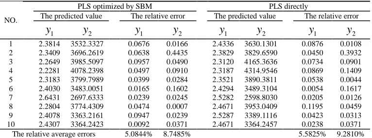
Table 2 the effect comparison between PLSR optimized by SBM and the simple PLSR in the experimental data of the traditional Chinese medicine

NO.

PLS optimized by SBM PLS directly

The predicted value The relative error The predicted value The relative error

1

y

y

₂

y

₁

y

₂

y

₁

y

₂

y

₁

y

₂

1 2.3814 3532.3327 0.0676 0.0166 2.4336 3630.1301 0.0876 0.0108 2 2.3409 3696.2619 0.0638 0.4435 2.3829 3829.6590 0.0450 0.3932 3 2.2649 3985.5097 0.0957 0.0490 2.3120 4165.3636 0.0734 0.0901 4 2.2281 4078.2398 0.0497 0.0910 2.3187 4314.9546 0.0869 0.1409 5 2.3183 3799.7989 0.0399 0.0284 2.3521 3890.3811 0.0538 0.0044 6 2.4030 3483.0051 0.0165 0.1602 2.4294 3489.3104 0.0054 0.1617 7 2.6431 2697.6333 0.0239 0.0245 2.5282 2598.8030 0.0205 0.0126 8 2.2804 3774.4309 0.0474 0.0007 2.4671 3953.0409 0.1195 0.0459 9 2.4078 3363.2161 0.0947 0.0239 2.5287 3389.1116 0.0423 0.0313 10 2.4307 3364.2423 0.0092 0.0371 2.4671 3364.2457 0.0238 0.0371 The relative average errors 5.0844% 8.7485% 5.5825% 9.2810%

Table 3 The sample data of the tool wear test

NO.

x

₁

x

₂

x

₃

x

₄

x

₅

y

SBM 1 482.86 751 620.66 3.438 102.4 58 1 2 494.49 839 665.88 3.655 307.2 134 1 3 545.95 957 701.96 4.293 512 177 1 4 499.07 923 708.18 4.052 614.4 185 0.9828 5 398.54 745 595.75 3.544 716.8 186 1 6 443.4 781 691.43 3.721 819.2 188 0.8664 7 475.45 874 685.48 3.935 921.6 208 0.8842 8 478.01 927 761.19 4.026 1126.4 254 1 9 517.2 1069 800.1 4.46 1228.8 276 1 10 513.44 1064 822.9 4.326 1331.2 290 1

Then we utilize the same scheme to analyze the data of tool wear[14] ( table 3) , and reject the 4, 6 and 7 sample with the efficiency values falling below 1.According to the tool wear test,

y

and

x

₁

、

x

₂

、

x

₃

、

x

₄

、

x

₅ have a

2.2427 1.3656 1.7361 2.7593 0.8319

1 2 3 4 5

0.0002983

[image:7.595.147.466.116.243.2]

y

=

x

x

x

−

x

−

x

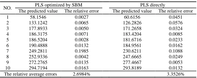
(11)

Table 4 the effect comparison between PLSR optimized by SBM and the simple PLSR in the data of the tool wear test

NO. PLS optimized by SBM PLS directly

The predicted value The relative error The predicted value The relative error 1 58.1546 0.0027 60.6156 0.0451 2 133.1242 0.0065 126.2826 0.0576 3 177.8933 0.0050 171.2658 0.0324 4 186.3175 0.0071 183.4204 0.0085 5 186.5204 0.0028 181.6716 0.0233 6 190.4888 0.0132 184.9561 0.0162 7 249.2811 0.1985 230.6211 0.1088 8 252.9336 0.0042 247.6665 0.0249 9 272.2765 0.0135 277.4667 0.0053 10 294.7194 0.0163 293.8189 0.0132 The relative average errors 2.6984% 3.3526%

In the table 2 and 4, using the relative average error as reliability criterion and referring to 2 dependent variables, we figure out the relative average errors by utilizing the PLS optimized by SBM algorithm are 5.0844% and 8.7485%, which is below to the results(5.5825% and 9.2810% )by using the PLS directly.According to the 1 dependent variable of the data of tool wear test, the relative average error optimized by SBM is 2.6984%, which is lower than 3.3526% calculated by the PLS directly.

CONCLUSION

Through the above analysis, we can obtain the following conclusions: Firstly, we propose to utilize SBM to optimize the PLS model, which improves the model precision and calculate the efficiency value of the sample points depending on SBM as well as analyze its characteristics, therefore, the “bad data” can be eliminated better and we obtain more reliable model finally. Secondly, comparing to the alone PLS, the relatively average error of PLSR optimized by SBM is lower. Thirdly, different DEA models have a variable effect on data samples, so we can adopt different DEA models to reduce the influence which invalid data have on the regression model. Fourthly, it is able to pull different DEA models into the regression model of the data of Traditional Chinese Medicine to provide better technical support to the Traditional Chinese Medicine.

Acknowledgments

This work is supported by the Key Laboratory of modern preparation of Traditional Chinese Medicine (TCM), Ministry of education and a national natural science foundation (61363042) and the National Key Basic Research Program of China (973 Program) (2010CB530602), This research also is supported by Jiangxi Province Innovation Foundation for Graduate (YC2013-S226).

REFERENCES

[1] Xu Qun. The research on non-linear regression analysis methods[D].Hefei University of Technology,2009. [2] Krishnan A, Williams L J, Mcintosh A R, et al. NeuroImage. 2011, 56(2): 455-475.

[3] Guo Jianxiao, Study on Improved High-Dimension and Nonlinear Partial Least-Squares Regression Method and Applications[D]. Tianjin University, 2010.

[4] Du J, Liang L, Zhu J. European Journal of Operational Research. 2010, 204(3): 694-697.

[5] Ma Shengjun, Wang Dongmei, Ma Zhanxin,et al. Journal of Inner Mongolia Agricultural University(Natural Science Edition). 2012, 33(1): 231-235.

[6] Cooper W W. Handbook on Data Envelopment Analysis[M]. Springer US, 2011.

[7] Wei Quanling. Data envelopment analysis model to evaluate the relative effectiveness —— DEA and network DEA[M].Beijing: China Renmin University Press, 2012.

[8] Chen J, Deng M, Gingras S. Computers & operations research. 2011, 38(2): 496-504. [9] Zhou Y, Xing X, Fang K, et al. Energy Policy. 2012, 57(0): 68-75.

[10] Li H, Fang K, Yang W, et al. Mathematical and Computer Modelling. 2013, 58(5–6): 1018-1031. [11] Tone K. European Journal of Operational Research. 2010, 200(3): 901-907.

[12] Sun Fenglin, Hao Zhifeng. Computer Engineering and Design,2010, 31(12): 2826-2829.

[13] Rodriguez J D, Perez A, Lozano J A. Pattern Analysis and Machine Intelligence, IEEE Transactions on. 2010, 32(3): 569-575.