STATE AND PARAMETER ESTIMATION
TECHNIQUES FOR STOCHASTIC
SYSTEMS
Matthew J. CARR
Centre for Operational Research and Applied Statistics
(CORAS)
University of Salford, Salford, UK
CONTENTS
Acknowledgements vi
Abstract vii
1. Introduction 1
2. Modelling background 6
2.1 Introduction 6
2.2 Parameter estimation 6
2.2.1 Maximum likelihood estimation 7
2.2.2 Alternative methods 11
2.3 Hazard and reliability 12
2.4 State estimation for discrete time stochastic systems 13
2.4.1 The conditional estimation problem 13
2.4.2 The least squares approach 17
2.4.3 Probabilistic stochastic filtering 18
2.4.4 The Kalman filter 20
2.5 State estimation for continuous time stochastic systems 25
2.5.1 Stochastic calculus and Brownian motion 25
2.5.2 Continuous time filtering preliminaries 27
2.5.3 Non-linear filtering for continuous time systems 29
2.5.4 An alternative approach 31
3. Recognising and measuring the potential for human error at
maintenance interventions using delay time modelling 33
3.1 Literature review 34
3.1.1 Modelling literature 34
3.1.2 Literature on fallible maintenance 36
3.2 Modelling and analysis 37
3.2.1 The basic delay time model 3 8
3.2.2 Modelling the injection of faults at PM 43
3.2.3 Simulating a process with potential fault injection at PM 48
3.2.4 Model specification and parameter estimation 50
3.2.6 Optimal maintenance policies with fault injection at PM 55
3.3 Numerical example 1 56
3.4 Aspects of human fallibility 68
3.4.1 Identification of the underlying process 68
3.4.2 Imperfect detection case (J3< 1) 69
3.5 Numerical example 2 71
3.6 Combining both aspects of human error 74
3.7 Discussion and further considerations 76
4. On-line modelling of fallible maintenance processes for complex systems using the delay time concept and probabilistic stochastic
filtering 82
4.1 Introduction 82
4.2 Preliminaries 85
4.3 Continuous time problem statement 88
4.4 Non-linear stochastic filtering (discrete-time, discrete-state case) 91
4.4.1 The filtering equations 91
4.4.2 Parameter estimation 95
4.4.3 Scheduling maintenance activities 95
4.5 Case 1 - basic scenario, x0 = 0 97
4.5.1 Modelling the process 97
4.5.2 The filtering expression pi(xt \ Nj) 99
4.5.3 Parameter estimation 100
4.5.4 Example 103
4.6 Case 2 - fault injection scenario, XQ > 0 105
4.6.1 The filtering expression p,{xi \ Nj) 105
4.6.2 Parameter estimation 106
4.6.3 Predictive equations 108
4.6.4 Example 108
4.7 A continuous time stochastic filtering representation 113
4.8 Summary and discussion 115
5. Condition monitoring and condition-based maintenance 117
5.2 Condition monitoring 119
5.3 Initial fault detection 120
5.4 CBM background 124
6. The proportional hazards model and a stochastic filter for condition
based maintenance applications 128
6.1 Introduction 128
6.2. The proportional hazards model 129
6.2.1 The hazard and reliability function 129
6.2.2 Modelling covariate behaviour 131
6.2.3 Parameter estimation 133
6.2.4 The conditional reliability function 135
6.2.5 The conditional failure-time distribution 138
6.3 Stochastic filtering 139
6.3.1 Introduction 139
6.3.2 The residual delay time distribution 141
6.3.3 Parameter estimation 143
6.4 Multiple indicators of condition 144
6.4.1 Principle components analysis (PCA) 144
6.4.1.1 Establishing significant principle components 144
6.4.1.2 Using PCA when modelling CBM 147
6.4.2 Dynamic principal components analysis (DPCA) 149
6.4.3 Independent components analysis (ICA) 151
6.5 Failure time analysis and replacement decisions 152
6.5.1 MTTF and MSB analysis 152
6.5.2 Replacement policies 155
6.6 Discussion 156
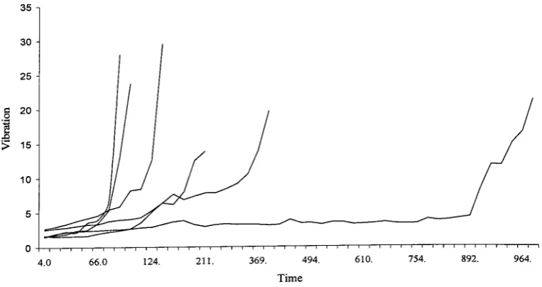
7. A case comparison of the PHM and a stochastic filter for a CBM
application using vibration monitoring 157
7.1 Introduction 157
7.2 The data 159
7.3 The proportional hazards model 160
7.3.1 The Weibull PHM 160
7.3.3 The conditional failure time distribution 162
7.4 The stochastic filter 163
7.4.1 The probability distributions 163
7.4.2 Parameter estimation 163
7.4.3 The conditional failure time distribution 165
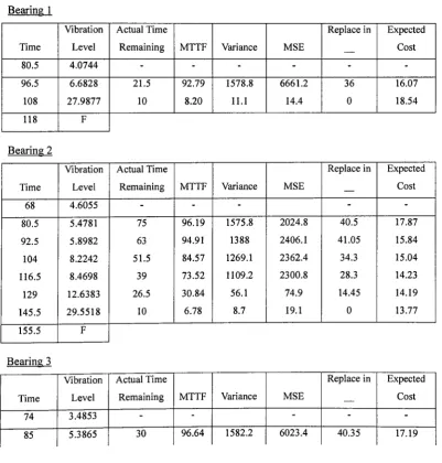
7.5 Results 165
7.5.1 Case 1 166
7.5.1.1 The proportional hazards model 166
7.5.1.2 The stochastic filter 171
7.5.2 Case 2 177
7.5.2.1 The proportional hazards model 177
7.5.2.2 The stochastic filter 180
7.6 Discussion 183
8. A case comparison of the PHM and a stochastic filter for CBM
applications using multiple oil-based condition monitoring parameters 187
8.1 Introduction 187
8.2 Oil data 189
8.3 Case study 1 191
8.3.1 Introduction 191
8.3.2 The data 191
8.3.3 The proportional hazards model 192
8.3.4 The stochastic filter 195
8.3.5 Results 198
8.3.6 Further 200
8.4 Case study 2 204
8.4.1 The data 204
8.4.2 Parameter estimation 206
8.4.2.1 The proportional hazards model - parameter estimation 208 8.4.2.2 The stochastic filter - parameter estimation 210
8.4.3 Comparing the models 211
9. Further stochastic filtering options for condition-based maintenance
applications 217
9.1 Introduction 217
9.2 EKF's for CM applications with limited computational power 218
9.2.1 A semi-deterministic extended Kalman filter (EKF) 219
9.2.2 A semi-deterministic EKF for residual life prediction using
vibration monitoring information 221
9.2.3 EKF for residual life prediction using vibration information
-example 222
9.2.4 Second-order extended Kalman filtering 227
9.3 Limited memory filter 229
9.4 Model combinations 231
9.4.1 Introduction 231
9.4.2 Fixed dynamics 232
9.4.3 Evolving dynamics 233
9.4.4 Example - fixed dynamics 235
9.4.4.1 Case 1 241
9.4.4.2 Case 2 243
9.5 Discussion 244
Appendix 248
Acknowledgements
I would like to thank my supervisor Professor Tony Christer who sadly passed away
earlier this year, for all the opportunities, support and guidance that he gave to me.
He is sorely missed, by myself, and everyone who knew and worked with him at the
University.
I would also like to thank my co-supervisor Dr Wenbin Wang for the support and
direction he has given to me during my PhD and beyond.
I also wish to thank Miss Susan Sharpies for her continuous support throughout all
my time at Salford.
To my parents, thank you for all your love and support.
ABSTRACT
This thesis documents research undertaken on state and parameter estimation techniques for stochastic systems in a maintenance context. Two individual problem scenarios are considered. For the first scenario, we are concerned with complex systems and the research involves an investigation into the ability to identify and quantify the occurrence of fault injection during routine preventive maintenance procedures. This is achieved using an appropriate delay time modelling specification and maximum-likelihood parameter estimation techniques. The delay time model of the failure process is parameterised using objective information on the failure times and the number of faults removed from the system during preventive maintenance. We apply the proposed modelling and estimation process to simulated data sets in an attempt to recapture specified parameters and the benefits of improving maintenance processes are demonstrated for the particular example. We then extend the modelling of the system in a predictive manner and combine it with a stochastic filtering approach to establish an adaptive decision model. The decision model can be used to schedule the subsequent maintenance intervention during the course of an operational cycle and can potentially provide an improvement on fixed interval maintenance policies.
construct relevant replacement decision models. The research is then extended to
consider multiple indicators of condition obtained simultaneously at monitoring
points. We conclude with a brief investigation into the use of stochastic filtering
techniques in specific scenarios involving limited computational power and variable
Chapter 1. Introduction
The general objective of the research documented in this thesis is to provide a contribution to the goal of optimising the performance of operational systems that are stochastic by nature and subject to some form of degradation over time. This categorisation incorporates almost any operational system from a complex industrial production line with many sub-systems to a simple photocopier or printer. The objective is achieved through the efficient scheduling of activities that are often overlooked as a viable means of boosting operational availability and performance, such as the use of planned preventive maintenance and effectively timed component replacements. These are activities that are often carried out in an opportunistic fashion when systems either fail (or are not currently operational for some other reason) or are conducted according to an inappropriate model producing decisions that are not cost effective or result in excessive downtime.
The particular focus of this research is on the techniques that assist in the characterisation of stochastic systems including both complex systems and individual replaceable components. Accurate representation of said systems is achieved through the use of an appropriate model specification and parameterisation. It is the parameter and state estimation techniques that are the primary topics of interest here. Using the constructed models, maintenance and replacement decision modelling can be optimised to reduce costs, identify areas of the current operational procedure that are lacking and limit the downtime of the system, thus increasing availability and operational efficiency.
maintenance interventions. We primarily consider the type of human error that manifests itself in the form of artificial fault injection during the course of planned inspection and preventive maintenance procedures although the model constructed is not limited to specifically human error based injections. The focus of the research is on the ability to characterise from relevant failure data, using an appropriate model specification and parameter estimation techniques, the fault arrival and failure processes of the system with emphasis being placed on the estimation of the level of fault injection that may be taking place. The subsequent modelling of complex systems concerns the on-line estimation and characterisation of the underlying fault arrival process using stochastic filtering and a hidden Markov model formulation. Modelling the system in a dynamic manner allows for the construction of adaptive decision models rather than fixed interval maintenance policies.
are also addressed and finally, some theoretical developments on the use of filtering
theory in the context of CBM are introduced in the final chapter of the thesis.
The outline of the thesis is now discussed;
Chapter 2 documents the necessary modelling and theoretical background and
presents the key introductory points for the techniques that are applied in subsequent
chapters.
Chapter 3 covers research undertaken regarding the provision for human error in
maintenance models of complex systems using delay time modelling; Initially a
discussion of the relevant delay time modelling and general modelling background
and literature is presented. Then the work undertaken using maximum likelihood
estimation to capture the necessary parameters is documented. A number of case
studies are presented to demonstrate the application of the proposed techniques and
the ability to compare differing model forms and combinations of the different
aspects of human error during inspection and maintenance procedures is also
addressed.
Chapter 4 is a continuation of the fault injection work contained in the previous
chapter. Initially we present an alternative description and solution methodology for
the problems addressed in chapter 3 by combining delay time modelling and a hidden
Markov model (HMM). The ability to construct adaptive decision models that
respond to the failure history of the system is of particular interest in this chapter.
Chapter 5 contains a discussion of relevant CM techniques and some associated
literature. We then document the necessary CBM literature that is available for
individual components and discuss the differences when modelling information that is directly or indirectly related to the underlying state of the component.
Chapter 6 presents two models for condition-based maintenance applications that are compared for industrial case studies in subsequent chapters. The techniques described are the proportional hazards model and a probabilistic stochastic filtering approach. We consider the potential for utilising multiple information sources and the need for data reduction techniques, such as principal components analysis (PCA), is addressed. The chapter concludes with a discussion of additional means of tackling some of the problems raised. These techniques include dynamic principle components analysis (DPCA) and independent components analysis (ICA). Techniques for comparing the models and establishing optimal replacement decisions are also introduced in this chapter.
Chapter 7 is a case comparison of proportional hazards modelling and probabilistic stochastic filtering when applied to vibration based CM information.
Chapter 8 is a comparison of the PHM and the filtering approach for condition-based maintenance applications using oil-based CM parameters. In this chapter, we also discuss the use of incomplete condition monitoring information and the impact on both parameter estimation and the ability to compare the two techniques.
The thesis concludes with a list of the associated references that are cited within the
Chapter 2. Modelling background
2.1 Introduction
In this chapter, the necessary modelling background and preliminaries for the research documented in subsequent chapters is presented. The techniques used for estimating the parameters of the various stochastic models developed in the thesis are introduced in section 2.2, section 2.3 introduces the hazard and reliability functions for systems that will fail at some unknown time and sections 2.4 and 2.5 introduce some of the techniques that are available for estimating the underlying state of discrete time and continuous time stochastic systems, respectively. The references and background that are relevant to the research on complex systems are given in the introduction to chapter 3 and those pertaining to the research on the monitoring of individual components are given in chapter 5. However, there are some general references that have been particularly useful in the development of the research contained here and these are now introduced. For information on system identification and related topics, see Ljung (1999), for state space models and the Kalman filter, the primary references have been Harvey (1989) and Jazwinski (1970), and for further non-linear stochastic filtering information, see Krishnan (1984), Jazwinski (1970) and Kallianpur (1980). Other general references have been Bernardo & Smith (2000) for background on Bayesian inference and analysis and Aoki (1967) and Liptser (1997) for information on control theory for the stochastic systems considered here.
2.2 Parameter estimation
all the relevant and required information from the data under investigation. The first
statistical property of an estimator that we consider is the level of bias, which is the
difference between the expected value of a parameter given by an estimator and the
true underlying value of that parameter. Amongst the class of unbiased estimators
for a given problem, an efficient estimator is the one with a minimal variance and as
such, a minimal mean-square error (MSB). An additional property for consideration
is that of consistency. A consistent estimator is one that converges probabilistically
to the true value of a parameter with an increasing sample size. In fact it is often
necessary to consider the asymptotic (large sample) properties of estimators when
selecting an approach for practical scenarios.
2.2.1 Maximum likelihood estimation
The models used in the research presented in this thesis are characterised by
parameters that are estimated from data using an appropriate modelling approach and
maximum likelihood estimation. The maximum likelihood estimates of the
parameter set are the values that maximise the likelihood function but they may not
necessarily be unbiased estimates. The bias of ML estimators may be quite large and
the estimator may not be unique or even exist for particular cases. Under the
regularity conditions that the first and second derivatives of the log-likelihood
function must be defined and the Fisher information matrix must not be zero, the
MLE can be considered to be asymptotically optimal, see Kendall & Stuart (1979).
For instance, the estimate is asymptotically unbiased in that the bias tends to zero as
the number of samples gets large. This property is a result of the fact that the
distribution of the estimate tends to a Gaussian distribution as the sample size
Cramer-Rao lower bound which is an asymptotic lower bound on the variance of any unbiased estimator.
If x is a continuous random variable with probability density function f(x;0), where 0 = 0i,02 ,...,0/c is the set of A: parameters under scrutiny, the likelihood of observing
the information set x = x\,X2,...,xr is given by the product
si*) = n/(*/#)
[2.1]Maximisation is often eased by taking logarithms of the likelihood function. The optimal parameter estimates are equivalent under either function. The log-likelihood function is
1(0 \x) = [2.2]
1=1
The maximum likelihood parameter estimates are then obtained as the simultaneous solutions of the k equations
dl(0 x) = 0
[2.3]
for7 = 1, 2, ..., k. The covariance matrix for the estimated parameters is established as
Z =
d 2 l(9 1 x) d 2 l(9\x) Q0* '" 60} d0k
d 2 l(0\x) d 2l(0\x) d9k d9, '" dffS
[2.4]
of the individual probability associated with each observation. In chapters 6-8, the
observed information is assumed to be conditional on previous observations and as a
result, the standard approach is to establish the likelihood of observing the r pieces of
information as the product of conditional probabilities, see Harvey (1989). The
functional form of the likelihood function becomes
*2>*i )>< */(*/ \xr-i,xr_2 ,...,x2 ,xl ) [2.5]
where, f(a \ b) is the probability of observing event a given that event b has already
been observed.
With the likelihood function in hand, an optimisation algorithm is still required for
maximisation of the expression with respect to the unknown parameters. In general,
a local optimisation method is designed to generate a sequence of points that will
converge to a local minimum. The algorithm is stopped or the sequence terminated
once a convergence criterion or criteria are met. Often a criterion is that the norm of
the gradient is small because theoretically at a local minimum the norm of the
gradient is zero. One approach that is available is the Broyden-Fletcher-Golfarb-
Shanno quasi-Newton (BFGS) algorithm. The BFGS algorithm is based upon the
second order Taylor polynomial of the objective function and the Newton-Raphson
method and has a convergence rate that is much faster than other optimisation
algorithms such as conjugate gradient methods. This is due to the fact that the search
directions for the BFGS are often more accurate however, more computational power
is required for each iteration. The approximate second order representation for the
log-likelihood function is
1(0 \x) * l(a\x) + Sa T Vl(a\x) + -Sa T H(0\x)Sa [2.6]
H(0\x) =
~d 2 l(0\x) 80^
8 2 l(0\x)
d 2 l(9\x)\ 60l d0k
8 2 l(0 \ x) 90k d0l '" d0k 2
[2.7]
are evaluated at 0 = a and da = (Sal ,...,Sak ) T is 0-a . The well-known Newton-
Raphson method for solving Vl(0 \ x) = 0 is given by the algorithm
where, c is the index. /l (c) is defined as an approximation to the inverse Hessian
matrix [//(# | x)]" 1 The Hessian matrix is the square matrix of second partial
derivatives and is often used in optimisation algorithms. This is due to the fact that if
the Hessian is negative definite at a critical point (when the gradient of a scalar
function is zero), then we have a local maximum. The inverse of the Hessian matrix
also gives the variance-covariance matrix for the estimated parameter values.
The BFGS algorithm is
A aa
ab_ T +ba T
(a Ag ^ ) [2.9]
where, q = 0 (c+l) -0 (c\ b = A (c) Ag {c) and
\x) p.10]
When the algorithm converges, the optimal parameter estimates are obtained. The
BFGS algorithm is presented here and used in the proceeding research in preference
to other candidate solutions to the optimisation problem, such as the Davidon-
Fletcher-Powell (DFP) method, due to the fact that it is widely regarded as being the
2.2.2 Alternative methods
In this section, we will discuss some (but by no means all) of the alternatives to
maximum likelihood estimation. An alternative and frequently used means of
estimating the parameters of a stochastic model or probability density is the least
squares approach which involves the minimisation of the squared errors between the
observed information and the model or density expectation. However, unlike
maximum likelihood estimation, probabilistic statements can not be made about the
estimated values using the least squares approach. A method similar to the least
squares approach involves the minimisation of the chi-square function using the
expectation from the model or density, see Kendall & Stuart (1979). Another
technique is the Rao-Blackwell theorem, see Rao (1965), that utilises sufficient
statistics for a given data set and modifies existing estimators to find an improved
estimator. A sufficient statistic is an observable random variable constructed from a
set of data that provides enough information to construct the conditional probability
distribution for the data set and is not a function of the population parameters.
Applications of the Rao-Blackwell theorem often use a maximum likelihood
estimator as a starting point. Alternatively, if the original estimator is unbiased and
complete then, according to the Lehmann-Scheffe theorem, the Rao-Blackwell
technique provides a means of finding the minimum unbiased estimator.
Another parameter estimator is given by the generalised method of moments which,
as the name implies, is a generalisation of the method of establishing the moments of
a probability distribution. In principle, it is similar to the minimum chi-square
estimator. Minimum variance unbiased estimators also exist however, although
theoretically sound, the restrictions placed on the bias can easily produce unrealsitic
estimates are obtainable with the availablility of prior information, see Sorenson
(1980). The MAP estimates are achieved by maximising the product of the
likelihood function and an a-priori probability distribution for the parameter.
Another technique that utilises prior distributions for the parameters is the
expectation-maximisation (EM) algorithm which is a recursive procedure that
defines some of the unknown information as latent variables and can also utlise the
likelihood function in aquiring optimal estimates. In terms of constructing
probability distributions, some techniques are available which do not require
parameterisation. The Kaplan-Meier approach is a nonparametric technique for
survival function estimation based on data only, see Kalbfeisch & Prentice (1973).
2.3 Hazard and reliability
The hazard and reliability functions are often utilised in applications involving the
analysis of the expected life of a system. For a given system or individual
component, we define/(O as a continuous failure time distribution on t > 0, and the
reliability function R(t), also known as the survival function, is the probability that
the system survives beyond time t. We have the relationship
/Z(r)=l-F(r)
[2.11]
where, F(t) is the cumulative failure time density given by F(t) = \ f(s)ds. The
hazard h(f) is often referred to as the instantaneous failure rate and is given by
h(f)=f(t)IR(t) [2.12]
We also have
F(0=l-exp{-//(0} [2.13]
where, H(f) is the cumulative hazard at time t given by H(t) = \ h(s)ds. Using
[2.14] Chapters 6-8 utilise a proportional hazards model (PHM) for determination of the life expectancy of individual components. In a general sense, to establish the hazard, the PHM weights the impact of the unit's age and the input from monitored information that is assumed to be in some way related to the degradation of the component. The hazard for the PHM is given by
[2.15] where, ho(t) is a baseline hazard function that is dependent on the age of the system only, y represents the information available about the system at time t and h(yy) is a function of y with a co-efficient y . The function A can be extended to incorporate the information from multiple sources (denoted by the vector y) as A,(yjy). In chapters 6-8, the PHM is investigated as a methodology for condition based maintenance applications and its derivation is contrasted with the technique of stochastic filtering that is used in this context as a probabilistic approach to the problem that arises from the methodology outlined in the next section.
2.4 State estimation for discrete time stochastic systems
2.4.1 The conditional estimation problem
information consists of failure times and the number of defects removed during the
course of planned preventive maintenance interventions. The modelling objective is
the characterisation of the underlying dynamics of the system regarding the fault
arrival process and the potential for human error related fault injections, with a view
to improving a given process and establishing a fixed decision model. As such, the
underlying (unobservable) state is the number of faults that have arisen in the system
by that point in time. However, in the context of condition based maintenance (see
chapters 5 - 9), the state of an individual unit is not easily definable and we are
required to consider variables that are related to or are functions of the severity of a
fault at a given moment, or functions of the general operational capability, such as,
the remaining useful life of the component before the defect leads to failure.
Monitoring techniques such as vibration monitoring and oil analysis provide the
indicator information that is used to estimate the state.
Techniques such as statistical process control (SPC) are limited when considering
data that is non-stationary and evolving stochastically. One of the techniques that is
suitable for data of this type is the stochastic filtering approach to state estimation
that utilises any knowledge of the system and the characteristics of the particular
indicatory information that is in use. The filtering approach assumes a statistical
description for the system and the observation noise (measurement errors) and
incorporates any uncertainties in the dynamics of the system. The recursive filtering
process is relatively straightforward for systems that are characterised by linear
relationships and perturbed by Gaussian white noise, (Harvey, 1989). The
methodology can be generalised into a general Bayesian filter using a probabilistic
approach and relaxing the linear assumptions to reveal an optimal filter designed to
and Jazwinski (1970). As such, it can be demonstrated that the linear filter is merely
a special case of the general non-linear filter. However, by relaxing the assumptions
of normally distributed noise and linear system equations, the computational
complexity is greatly increased and approximate or numerical solutions are required,
as is illustrated in chapters 4, 7 and 8. An understanding of multivariate random
variables, Gaussian distributions, white noise processes, conditional probabilities and
Bayes' theory are of particular relevance to the proceeding research. In this section,
we focus on the discrete time state estimation problem where, information is received
and knowledge of the state is updated at discrete time points during the life of the
system or component. The estimation problem is addressed using the least squares
method and a probabilistic filtering approach for a general state and condition input
where, the state and observation processes are described by vector processes.
An important element of the discrete probabilistic filtering approach is the Markov
property of independent increments that implies that current states are independent of
their history and as such, future states may be inferred solely from knowledge of the
current state vector. For discrete time systems, the conditional probability density
function
P(xi+ i |*o»*i'-»*/) = P(XM I*/) P- 16]
describes the transition for a state vector x from one stage to the next where, in some
applications, the stages may correspond to monitoring intervals. Using the transition
densities, the state at the next discrete time point * /+1 can be modelled as the
conditional mean
Many stochastic systems can be modelled effectively using a first-order Markovian
discrete time representation of the form
*/+ i=/(*/,'/+i) + v/ [2.18]
where, /,- is the age of the system at the fth check-point and v, is a random
disturbance that is often assumed to be normally distributed and independent in time.
The expression describing the evolution of the stochastic process, equation [2.18], is
used in control theory with the inclusion of an additional control input M,
as /(*»>'/+!>«/) See Aoki (1967) for details on control theory for discrete time
stochastic systems.
The observed information vector y is assumed to be a function of the state of the
system and a level of measurement noise e t is incorporated in the observation
expression as
y.=h(x i ,ti ) + e i [2.19]
When considering systems where the observed data is not directly related to the state
or condition that is the objective measure of the estimation (filtering) or prediction
process, the observations and the state are assumed to be correlated stochastically
and in many estimation problems (see the hidden Markov modelling undertaken in
chapter 4), it is a necessary requirement that the subsequent state xi+\ may be
determined uniquely from the current state x/ as
P(XI+I I */>£,) = P(*M I */) t2-20]
where, the state and measurement noise are assumed to be mutually independent.
However, it is often possible to transform the situation when the assumption does not
form. See Harvey (1989) for details. The conditional mean can be used to estimate
the condition x when an observation y is obtained as
'* t \y t } = J*,/fe, I >,)«/*,= -' -'-' dXi = '-"-"'-'' -' [2.21]
— / J * —/ * J r\(-\i \ — r../— .. \ J
assuming that the various probabilistic relationships are defined. The conditional
mean gives the mean square optimal estimate, however, it is complicated to update
for dynamic systems, see Jazwinski (1970). A notable exception is that of linear
systems perturbed by Gaussian noise where, the approach using the properties of
conditional mean estimation is known as the Kalman filter. Estimation and the
resulting analysis is far less complex when considering linear estimates, the Linear
Least Mean Square (LLMS) estimation process produces results identical to the
conditional mean approach for Gaussian distributed random variables. The LLMS
approach involves the estimation of a and b in the expression xt = a + byi to find the
parameter values that minimise the error covariance. However, the LLMS filter only
gives optimal estimates in the special linear case described.
2.4.2 The least squares approach
We now consider a general least squares approach to the state estimation (not
parameter estimation) problem for the system and observation process described by
equations [2.18] and [2.19]. With the probabilistic stochastic filtering approach
described in the next section, the errors in the system and observation expressions are
defined as random inputs with known properties. However, when applying the least
squares approach, they are defined as merely errors of an unknown quantity.
Assuming that an estimate of the initial state *0 is available, upon the availability of
[2.22] with respect to {*0 ,...,x, ; Vi, >v,-} and subject to the constraints
'i+i) + v* [2.23]
for k = 0,1,..., /-1. In this context, the contributions Pg 1 , Q~l and R^ are simply defined as weighting matrices. The series of estimated state vectors {x0 , x\,..., xt } that minimise equation [2.22] are the smoothed solution and xt is the filtering solution at time /,. The major drawback of the least squares approach is that upon observing each new vector of stochastically related information, y. , an entirely new problem must be solved. An alternative is the recursive least squares (RLS) algorithm involving the minimisation of JM in terms of y. and the estimate of the state from the previous recursion xt . Analogous to the least squares approach for estimating parameters, probabilistic statements can not be made about an estimated state using least squares state estimation.
2.4.3 Probabilistic stochastic filtering
When conditioned on stochastically related observations, an optimal estimate of the state is obtained using the following general framework for the majority of systems. Consider a non-linear stochastic system with state and measurement equations;
x , = f(x t- i v.) F9 941
— i+l I vi/''»+l'i;/ V--*-^\
y_i =*(*,-,',-) + «/ [2.25]
x t = E[Xj 1 Y_t ] which must be computed recursively. Firstly, using Bayes' rule, the
functional form of the conditional probability density function p(xf |7( ) must be
determined as
P(x.i,y. I £ M ) = p(x t | y^Y^pfy | 7 M ) = p(y. |* r ,F M )X* ; I I M ) t2 -26!
For the non-linear system defined in equations [2.24] and [2.25], the measurement
contains white noise and we may therefore assume that the estimated condition
contains all the necessary information regarding the measurements and as such, we
have
p(y i \x i ,Yi_l ) = p(y.\x l ) [2.27]
Using equations [2.26] and [2.27], the probability density function of a particular
state given the monitored condition history to date can be established as
p(y
I*,-)
P(xt \li) = ~' , />(*, I Lt-i ) [2.28]
p(yf
II M)
Using the transition density, the probability of a one-step predicted state is given by
where, all the densities can be conditioned on the observed data and due to the
Markovian nature of the process, the conditional predictive density becomes
P(*t I L-i) =
[2.30]
Combining equations [2.28] and [2.30] produces
. i
' \p(x i | x i_l )p(x i_l | ! M )</JC M [2.31] IM)
, ,
j
}p(yt
I *,
Equation [2.32] is the formulation used in chapter 4 and is adapted for a model with a
discrete state space. In chapters 6 - 8, the particular definition of the state as the time
remaining before failure provides a deterministic relationship between subsequent
underlying states and enables the updating equation
P(xt I */-i )/>(*M I I M ) = X*, I r/_i ) [2.33]
to be established.
For non-linear, non-Gaussian systems the conditional probability density given by
equation [2.32] is intractable and sub-optimal policies or approximations are required
to obtain an estimate of the state. For linear systems, the aforementioned Kalman
filter provides a convenient means of updating the conditional density using the
properties of the Gaussian distribution. In highly non-linear problems, it may be
desirable that the system be modelled continuously between observations. Defining
xt .+s as the estimate of the underlying state at time (f, + s), the system expression
that describes the evolution of the state is utilised as x(j+s = /(*,-, tit (tt + s)) for
2.4.4 The Kalman filter
There are a number of different ways of representing and deriving the Kalman filter
and the approach described here is based on the propagation of the conditional
distribution. The Kalman filter may be applied to any linear system model in the
state space form, see Harvey (1989) and Aoki (1967) for extensive information on
the Kalman filter in the probabilistic framework and the augmentation of state
Although the various definitions of state in this thesis are univariate, here we present
the matrix form of the linear system expressions and the Kalman filtering equations
in order to provide the appropriate background for the development of approximate
Kalman filters applied to non-linear systems in chapter 9. Consider the following
observation expression in the state space form for a system observed at equidistant
time points;
£,=£/*/+*, [2.34]
where, the vector y_ has N elements and H is a time dependent matrix of dimension
(Nxm). The underlying state is then defined as a first-order m-vector Markov
process
*,-+ i=£,*,-+G/«/+v/ [2.35]
where, F is an (mxm) time dependent matrix. The contributions v, and Cj are TV-
vector white noise processes that are assumed to be mutually independent and the
(ax 1) vector u is a control input such as, the effect on the system state of a
maintenance intervention with a time dependent matrix G of order (mxa). It is
assumed that the control input is to some extent within the control of the user and
that the effect is either known or determined uniquely from knowledge of the
observations. However, one cannot always be certain of the effects that may arise as
a result of actions taken and attempting to quantify the impact of maintenance
procedures can prove difficult. The control is usually derived subject to some
criterion function and is often used in control theory to obtain some type of balance
when deviations in the estimated value of the state are occurring, see Aoki (1967).
The units of the control function are likely to be shared by the state that is the focus
of the particular filtering application. For instance, if the state of the system is taken
corrective action taken at maintenance interventions may result in a decrease in the
systems virtual age and as such, an increase in the residual life would be expected.
The notation tt is defined as the time of the /th iteration of the filtering process that,
in the context of a maintenance process, could represent an intervention or
monitoring point. Assuming that 7, represents all the available information at tj
including any control actions taken and that the objective is to ascertain the state at th
the problem is one of prediction when (, < tt, filtering or estimation when (, = tt and
smoothing or hindsight when tj > /,-. The covariance of the estimation error is given
by
P l[j=ElXi-xl[j]\xl -x,v]T P.36]
where, x,y represents the optimal estimate. As noted previously, the LLMS estimate
and the conditional mean propagation approach derive identical results for this
scenario under different assumptions. This is due to the fact that, the LLMS estimate
is reliant on the assumption of white noise disturbances and coincides with the
conditional mean for Gaussian distributed data. Here, we consider the system
described by equations [2.34] and [2.35] and assume that both the measurement and
system disturbances are 0-mean Gaussian white noise processes and mutually
independent as
For most of the estimation approaches used in this research, some prior knowledge of
the initial state or condition of the system is required and it is often a requisite that
this initial state has no relationship with either of the noise sequences included in the
model. With this particular case, we assume the initial state to be normally
estimation and prediction purposes, given the available information, are also taken to
be Gaussian;
X*,IZ,)~;V(*,,£,) [2.38]
P(*i+i I !,) ~ tf(*/+ i|/,£>n/) [2.39]
and the parameters are obtained using the Kalman filtering process. The expressions
are presented in two stages for prediction and updating purposes. The prediction
equations that are used between observations are
xl+]V =F l xl +Gi u i [2.40]
p. ... = F P F T +R [2.41]
f_/+l|j i_;i_;i_; ^ £i l J
The updating equations upon observing the next piece of information are
*]
[2>42]
where, the Kalman gain function is
The system is initialised using the mean and variance of the prior distribution for the
initial state. Parameter estimation for the Kalman filter is undertaken using the
conditional probability of observing each piece of information to formulate the joint
density. The parameter values are then obtained using the maximum likelihood
approach discussed earlier in this chapter. See Harvey (1989) and a furnace erosion
prediction case study in Christer et al (1997) for more details of the parameter
estimation process for the discrete Kalman filter.
As noted previously, when considering non-linear systems (as all the scenarios
required for estimation and prediction of the underlying state. Applying an extended
Kalman filter (EKF) to non-linear systems essentially involves applying the standard
Kalman filter to linearised versions of the non-linear systems (see chapter 9 for
details). There are many variations on the EKF in the literature. For instance, the
'iterated' EKF is designed to consider situations where it is not obvious what the
relevant linearisation point is when computing the Kalman gain function. The
process involves iterating over the measurement equation and the iteration means
that the linearisation point is changed. In some situations, this modification can
result in improved performance of the filter, (Jazwinski, 1970).
Another variation on the basic EKF is a 2nd-order EKF where, the recursive
procedure deals with the 2nd-order terms in the Taylor series expansion of the state
expression. See chapter 9 for details. The resultant equations contain quadratic
terms that are replaced by their expected values. Gaussian sum estimators are
frequently described in the literature available on approximate non-linear state
estimation techniques. The complexity associated with the recursive computation of
the conditional density functions is simplified through approximation. The method
involves approximating an arbitrary density function by a weighted sum of Gaussian
distributions. The process of propagating the conditional means and covariance
matrices involves applying a number of EKF's simultaneously and weighting the
respective output. To ensure that the covariance matrices are small, it is a general
requirement that a large number of filters are used in achieving the best possible
approximation. The primary approach pursued in the research presented here is the
probabilistic approach whereby, the characteristics of the various relationships and
the associated error processes are described by probability distributions. For the
problem is attainable however, an analytical means of solving the expression is not
and approximate or numerical techniques are required.
2.5 State estimation for continuous time stochastic systems
2.5.1 Stochastic calculus and Brownian motion
In this section, we are concerned with modelling the state of a system or a
component as a continuous-time stochastic process {^/}o</«» A realisation of the
process X is called a sample path and is usually continuous however, jump
discontinuities are viable on the condition that the functions involved are right-
continuous. A necessary component of much of the continuous time non-linear
filtering theory is Brownian motion. A Brownian motion is a process that has
independent and Gaussian distributed increments with a mean of zero and an
incremental variance that is proportional to the size of the increment. This property
is attributable to the fact that each increment is comprised of many smaller,
independent sub-intervals. Brownian motion is utilised in Ito processes (or
diffusions) which are the primary tools in stochastic calculus. An Ito process is
described by a stochastic differential equation
dXt =Ut dt + Vt dWt [2.45]
where, {W,} is a Brownian motion. For a small time increment At, we have
Xt+At -Xt ~N(U,At ,V?At) [2.46]
where, the Gaussian distribution is conditioned on the processes W, U, V and X over
the interval [O,/]. The process U represents the rate of change inland V represents
the level of random diffusing. Both U and V are assumed to be non-anticipating or
adapted processes. The adaptive property means that they are not reliant on the
until that point. With V being an adapted process, the stochastic integral of X can be
given with respect to a Brownian motion W as
Xt = \Vs dWs = li
0 " /=!
p.47]
The limit is very complex in most situations and indeed often does not exist.
However, the limit always exists in quadratic mean or if the adapted process has
bounded variation. The Ito process given by equation [2.45] can be expressed as a
sum of stochastic integrals as
/ t
X,=XQ + Jt7, ds + \VS dWs [2.48]
o o
For X, =f(t, Wt), partial differentials are taken to ascertain the change in the rate of
the process as
dXt = ft (t,Wt )dt + fw (t,Wt )dWt + fww (t,Wt )dt [2.49]
and this is known as Ito's lemma. Equation [2.49] can be written in the form of a
stochastic integral as
t tj i N
Xt = X0 + \fw (S,Ws }dWs + I ft (s,Ws ) + -fww (s,Ws ) Ids [2.50]
o
(A
L
j
where, the final term is included because even squared increments of a Brownian
motion can have an impact on the overall process. Another integral form that is
available for stochastic processes is the Stratonovich integral which can be expressed
in terms of the Ito integral. Although, it is a useful approach for problems involving
stochastic differential equations, it lacks some of the necessary properties that are
required for stochastic filtering, see Krishnan (1984) for details.
Y,=h(t,Xt ) [2.51]
The change in the observation process is described by
dYt = ht (t, Xt )dt + hx (t, Xt )dXt + i hxx (t, Xt )(dXt } 2 [2.52]
where, (dXt ) 2 = V 2 dt is the quadratic variation of X. In keeping with the
description of the observation process, a stochastic differential equation for a general
Ito process Xt is given by
dXt = /(/, Xt )dt + g(t, Xt )dWt [2.53]
for functions/and g that are dependent, in this context, only on the current value of
the process X. Meaning that the process is of a Markovian nature where,/and g are
analogous to the transition probabilities of a Markov chain. A further important
element of the stochastic calculus discussed here are martingale processes. A
process X, is a martingale if for t < u, E \XU \ Xs ,0 < s < t] -Xt and as such, the
expectation is E[JTJ -E[^"0 ] for all t. An Ito process is a martingale if it satisfies
the property dXt = VtdWt . Importantly, Brownian motion is itself a martingale and
can be expressed as
Xt = \Vs dWs * £ P,M (Wt . - Wt.^) [2.54]
o »=i
t
where, the expectation is E[Xt ] = 0 and E[X?] = J E[V 2]ds. o
2.5.2 Continuous time filtering preliminaries
Liptser & Shiryaev (1989) show that, if the state is governed by a stochastic
differential equation and the process describing the evolution of the state over time is
representation. An Ito process can be represented as a diffusion process relative to
the innovations process V. In the filtering representations discussed here, the
innovations process is a Brownian motion process that represents the new
information that is available and consists of the differences between what is expected
to be observed and what is actually observed. The innovations process is derived
with respect to the cr-field generated by the observation process $ and is crucial
when deriving the non-linear filtering representations. The innovations process is an
^-martingale, this property is implied by the fact that the innovations process is
assumed to be of the Brownian motion type. Doob's decomposition theorem also
illustrates this property and Kallianpur (1980) gives a more in depth discussion of the
innovations process.
We are concerned with the estimation of the state (Xt, teT] of a system with respect
to a cr-field. As with the problem scenario for the discrete time case in section 2.4,
the state is not observable directly and must be ascertained via an observation
process that is assumed to be correlated with the state. In contrast to the discrete
time case, we are interested in updating our knowledge of the state continuously as
observations arrive continuously. The state estimates are derived using the
observation process and an optimal criterion such as the MSB function. As with the
discrete systems, the conditional expectation of the state provides an optimal
estimate for most criterion functions however, the expectation will in general be a
non-linear function of the observations. The issue is further complicated by the fact
that both the state and observation process are assumed to be governed by stochastic
differential equations and the resultant expression for the conditional expectation of
the state will also be a stochastic differential equation. For non-linear cases, the
as such, approximations or sub-optimal policies are required. The linear scenarios
require only the second moments of the conditional density and therefore the
evaluation of the conditional mean is a tractable problem. Analogous to the
treatment of discrete time systems, the estimation procedure for linear systems can be
derived within the framework of a general non-linear model, see Krishnan (1984).
Using the properties of martingales, a closed-form representation for the general non-
linear stochastic system is given by Liptser, Krishnan (1984) and Kallianpur (1980)
and some approximation is required to obtain the estimate. Under general
conditions, any martingale can be given as a stochastic integral. Krishnan (Theorem
8.4.1) shows that a square integrable martingale can be given as a stochastic integral
with respect to the innovations process and it is this fact that makes the closed-form
representation possible.
2.5.3 Non-linear filtering for continuous time systems
We are considering the complete probability space (Q $, P) and are attempting to
compute the least squares estimate of the state of the system {X,, teT} given the
availability of the current value and history of the observation process {7,, s < t,
teT} and as noted previously, this involves finding the conditional expectation of the
state given the cr-field generated by the observation process {<F,, teT}. Further, we
require that the conditional expectation be updated recursively and continuously.
The state of the system adheres to the process {Xt, J3,, teT} and is taken to be an Ito
process defined on the complete probability space as
The observation process {Y,, /?,, t&T} is also an Ito process and is defined on the
complete probability space as
t
Y,=X0 + JX dT + Vt [2.56] o
where, unique solutions exist for both the state and observation at time t and Xo is an
arbitrary initial condition that is assumed to be independent of all processes involved
in the system equations, {/?,, teT} is the filtration cr-field defined by
/3( iDcr{X0 ,Xs ,Ws ,Ys ,Vs ,s<t,teT} and $= a{Ys,s < t, teT} is the filtration
a-field generated by the observation process, where ^ c /?,. The state and the
observation process are defined as semi-martingales on the cr-field /?/, and/ and ht
may be functions of X, and are /7rmeasurable. Finally, W, is a general right-
continuous martingale process and {Vh /3t, t&T} is a Brownian motion process with
parameter crv. The innovations process v, has the same statistics as V, and is given by
dvt =dYt -ht dt [2.57]
where, the cr-field generated by the innovations process is equal to the cr-field
generated by the observation process. The same representation for the non-linear
filtering theorem can be derived without this assumption but the derivation is much
more complex.
The conditional estimate for the state of the system with respect to the cr-field at time
/ is given by
1
dXt =ft dt
-dt
or as a sum of integrals as
dvT [2.59]
where, (W,V), is the quadratic covariance between W and V. However, as noted
previously, this expression is generally intractable except in the linear Gaussian case.
See Krishnan (1984) and Kallianpur (1980) for proofs of the filtering theorem. A
useful modification is to consider the error quantities XT = XT_ - XT_ and
hT = hT_ - hr_ that enable the representation
1
2 ^ dvt [2.60]
If Wand Fare independent martingales then (W,V^ = 0 and the filtering expression
becomes
dXt =ft dt + — E 3l (X,ht )dvt [2.61]
which is a useful representation for many cases. Krishnan (1984), Kallianpur (1980)
and Liptser & Shiryaev (1989) present very similar treatments of the filtering
problem from a martingale perspective. Engineering applications including Koch
(1986) tend to utilise a Poisson counting process with independent positive
increments as
N, = No + *t + mt [2.62]
where, N, is the number of events and mt is a martingale.
2.5.4 An alternative approach
An alternative approach to the continuous conditional estimation problem involves
partitioning the range [0, t] into sub-intervals AQ = 0, A\, A2, ..., An - t. Then,
,y.,y_A >->y_A
)
[2.63]
H » 00
for the continuous information path Yt ={y ;0<s<t}. Redefining the
observation expression in a manner consistent with the probabilistic framework
developed in section 2.4.3, we have
0 + dt] [2.64]
where, E(drj dtj ) = Q(t)dt for Q(t)>Q, and p(XQ ~) is assumed known and
independent of 77 . To establish a conditional density for the underlying state at time
t, the approximation
£xexp
-~\h(Xs , S)T Q-\S)h(Xs ,s)ds+[
2 o o
can be used where, the expectation is taken over {Xs ;0<s<t}.
Chapter 3. Recognising and measuring the potential for human
error at maintenance interventions using delay time modelling
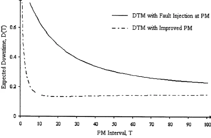
Within the context of Delay Time modelling, we investigate an approach whereby
the injection of defects at maintenance maybe ascertained from basic inspection and
failure data. The model is developed in the context of a competing risks scenario and
the objective of the research is not to assist management in optimising existing
situations that incorporate substandard procedures but rather, the intention is to
highlight the existence of such inefficiencies and to demonstrate the benefits that
may be achieved through improved practice. Although the model is constructed with
the provision for human error based fault injection in mind, the structure of the
model does not limit its application to situations that incorporate specifically human
error. The form of the model is appropriate for scenarios incorporating any kind of
fault injection. A number of cases are investigated using simulated data to test a
methodology for establishing the existence and indeed the level of potential human
error injected faults. This entails the selection of an appropriate form for the model
and accurate estimation of the necessary parameters.
Initially, a review of the relevant background and supporting literature is presented.
The basic delay time model and the associated parameter estimation approach are
then introduced with a view to extending the modelling and estimation for the cases
incorporating human error. The impact of potential fault injection on the resulting
downtime modelling phase is discussed and the methodology adopted for simulating
the process and obtaining the necessary failure and preventive maintenance (PM)
repair information is introduced. Some modelling options are proposed and
implemented on the simulated data sets and the ability to differentiate between a
assessed. The model selection approach is then extended and tested for comparison of models incorporating fault injection and models incorporating fallible detection of existing defects at PM. The chapter concludes with a discussion of general modelling recommendations, potential extensions to the work and the limitations of the modelling approach encountered.
3.1 Literature review
3.1.1 Modelling literature
For the research documented in this chapter, delay time modelling is used to represent the failure and inspection process for complex dynamic systems. The delay-time concept was first introduced in an appendix to Christer (1973) and then in a cost based decision model utilising subjective estimation in Christer (1982). The first formal presentation of the delay-time model for systems in a steady state of operation was given in Christer & Waller (1984a). Initially, the model was developed for systems with a homogenous fault arrival rate and then extended for the non-homogenous case. The paper also addressed the issue of non-perfect detection of existing faults at inspection. Industrial case studies include the application of delay time modelling to a canning line, Christer & Waller (1984b), and to the maintenance of coal mining equipment, Chillcott & Christer (1991).
sets only permit the accurate estimation of some of the model parameters using
objective methods, subjective input is required to establish the model of the system.
Christer & Waller (1984a) discussed the subjective estimation of delay time
distributions using expert opinion obtained from experienced engineers. Further
work on the subjective engineering-based estimation of delay time distributions can
be found in Wang (1997) and Christer & Redmond (1992) presented objective
parameter updating techniques for subjectively estimated delay time models. The
maximum likelihood estimation of optimal inspection intervals is addressed in Baker
et al (1997) and Christer et al (1998, 2000) considered parameter estimation
problems with either limited or deficient data sets. Christer & Wang (1992, 1995)
developed a delay-time model to represent the condition monitoring of a plant for the
single component case and subsequently, a multi-component system. Reviews of the
developments in delay time modelling can be found in Baker & Christer (1994) and
Christer (1999).
With regard to the type of physical process and preventive action under investigation,
Ascher & Feingold (1984) present an extensive account of maintenance techniques
for repairable systems. When modelling the impact of potential fault injection in this
chapter, the delay time model is presented in the context of the competing risks
model. See Bedford & Cooke (2003) and Crowder (2001) for information on
competing risks and the associated problems of parameter identifiability. Counting
processes are used to model the system failures as a stochastic process and a
thorough treatment of the Poisson process, and variations of, can be found in Ross
(1983). Barlow & Hunter (1960) give the initial presentation of the non-homogenous
systems incorporating negligible failure repair times, the type of failure process that
we consider in section 3.2 follows a NHPP in the limiting steady-state case.
3.1.2 Literature on fallible maintenance
Many studies have highlighted the presence of human error related defect injections
at maintenance interventions. Steedman & Whittaker (1973) estimated that in a
particular ICI plant, up to 30% of system failures were directly attributable to defects
injected at some point during the course of the previous PM. An ASRS air transport
report, Patankar & Taylor (2003), claimed that up to 40% of defects that are present
in an aircraft at any given time are due to the unintentional release of further errors
during substandard inspection and repair procedures. It is feasible that the inspection
or repair process for existing faults could result in the accidental injection of further
and potentially more severe defects. For instance, Jia et al (2002) encountered a case
where one specific error-prone maintenance procedure consistently produced defects
that subsequently resulted in a system failure. In cases such as this, it may be
beneficial to reduce the level of maintenance or indeed forgo it altogether and rely
solely on breakdown maintenance. Alternatively, the modelling and identification of
a defective process can reveal areas for potential improvement. In a limited PM data
and 'selective repair' case, Christer et al (1998), the modelling process revealed
defects that could potentially be removed and the resulting improvement in
maintenance procedures produced downtime savings of approximately 15%. This
illustrates the potential benefits of modelling human error, and although the focus of
that particular study was on the failure to identify and remove existing defects, the
quantities and levels of reduction in downtime are of interest.
Similar scenarios and alternative modelling solutions for problems that include