Path planning algorithm for a car like robot based on voronoi diagram method

PATH PLANNING ALGORITHM FOR A CAR LIKE ROBOT BASED ON VORONOI DIAGRAM METHOD

HAIDIE INUN

A project report submitted in partial

fulfillment of the requirement for the award of the Degree of Master of Electrical & Electronic Engineering

Faculty of Electrical & Electronic Engineering Universiti Tun Hussien Onn Malaysia

ABSTRACT

The purpose of this study is to develop an efficient offline path planning algorithm that is capable of finding optimal collision-free paths from a starting point to a goal point. The algorithm is based on Voronoi diagram method for the environment representation combined with Dijkstra’s algorithm to find the shortest path. Since Voronoi diagram path exhibits sharp corners and redundant turns, path tracking was applied considering the robot’s kinematic constraints. The results has shown that the

Voronoi diagram path planning method recorded fast computational time as it provides simpler, faster and efficient path finding. The final path, after considering robot’s kinematic constraints, provides shorter path length and smoother compared to

the original one. The final path can be tuned to the desired path by tuning the parameter setting; velocity, v and minimum turning radius, Rmin. In comparison with the Cell Decomposition method, it shows that Voronoi diagram has a faster computation time. This leads to the reduced cost in terms of time. The findings of this research have shown that Voronoi Diagram and Dijkstra’s Algorithm are a good

v

ABSTRAK

Kajian ini bertujuan untuk membangunkan satu algoritma perancang laluan secara luar talian yang cekap serta berupaya mencari laluan selamat yang optimum dari titik permulaan ke titik sasaran. Algoritma tersebut adalah berdasarkan

kepada kaedah gambar rajah Voronoi untuk mewakilkan persekitaran dan

digabungkan dengan algoritma Dijkstra untuk mendapatkan laluan terdekat. Oleh kerana laluan yang diperoleh menggunakan gambar rajah Voronoi mempunyai sudut-sudut tajam dan pusingan yang berlebihan, penjejakan laluan digunakan dengan mengambil kira kekangan kinematik robot. Hasil kajian menunjukkan

bahawaperancang laluan menggunakan kaedah gambar rajah Voronoi merekodkan masa pengiraan terpantas dan merupakan kaedah lebih mudah, lebih cepat dan cekap. Selepas mengambil kira kekangan kinematic robot, laluan yang diperoleh adalah lebih pendek dan licin berbanding dengan laluan asal. Laluan tersebut boleh ditala dengan menala parameter halaju, v dan jejari pusingan minimum, Rmin.

Perbandingan dengan kaedah Cell Decomposition, menunjukkan bahawa kaedah gambar rajah Voronoi mempunyai masa pengiraan yang lebih pantas. Ini membawa kepada pengurangan kos dari segi masa. Penemuan kajian ini menunjukkan

CONTENTS

THESIS STATUS APPROVAL EXAMINERS’ DECLARATION TITLE DECLARATION ACKNOWLEDGEMENT ABSTRACT ABSTRAK CONTENTS LIST OF TABLES LIST OF FIGURES

LIST OF SYMBOLS AND ABBREVIATIONS LIST OF APPENDICES

i ii iii iv v vi viii x

CHAPTER 1 INTRODUCTION

1.1 Background 1.2 Problem Statement 1.3 Objectives

1.4 Scope of the Project 1.5 Organization of Report

1 1 2 4 4 5 6

CHAPTER 2 LITERATURE REVIEW

2.1 Introduction

2.2 Classical Path Planning Methods

2.3 Representation technique in Path Planning 2.4 Cell Decomposition (CD)

2.5 Roadmap (RM)

2.5.1 Voronoi Diagram

vii

2.5.2 Probabilistic Roadmap

2.5.3 Rapidly-exploring Randomise Tree 2.6 Potential Field

2.7 Bezier Curve

2.8 Comparison of the method 2.9 Search Algorithm

2.9.1 Bread-first Search 2.9.2 Depth-first Search 2.9.3 A* Algorithm 2.9.4 Dijkstra’s Algorithm 2.10 Car-like Robot Model

2.11 Previous Study on Voronoi Diagrams

11 12 13 13 15 17 18 19 20 21 22 23

CHAPTER 3 METHODOLOGY

3.1 Introduction

3.2 Project Planning and development 3.3 Software Development

3.4 Voronoi Diagram Construction 3.5 Generation of Roadmap

3.6 Dijkstra Algorithm for Searching Shortest Path 3.7 Path Tracking Considering Robot’s kinematic Constraint 25 25 26 28 30 32 35 37

CHAPTER 4 RESULT AND ANALYSIS

4.1 Overview

4.2 Simulation Result

4.2.1 Case One (Environment with 10 Obstacles) 4.2.2 Case One (Environment with 20 Obstacles) 4.2.3 Case One (Environment with 30 Obstacles) 4.2.4 Case One (Environment with 40 Obstacles) 4.2.5 Case One (Environment with 50 Obstacles) 4.3 Result Conclusion

CHAPTER 5 DISCUSSION AND ANALYSIS 5.1 Introduction

5.2 Data Analysis

5.3 Comparison with Other Method 5.4 Discussion

53 53 53 56 60

CHAPTER 6 CONCLUSION AND RECOMMENDATION

6.1 Conclusion 6.2 Recommendation

62 62 63

REFERENCES APPENDICES

ix

LIST OF TABLES

4.1 Collected Data From Matlab (10 Obstacles) 42 4.2 Collected Data From Matlab (20 Obstacles) 44 4.3 Collected Data From Matlab (30 Obstacles) 46 4.4 Collected Data From Matlab (40 Obstacles) 48 4.5 Collected Data From Matlab (50 Obstacles) 50 5.1 Summary Of Calculation Time And Path Length For

Different Number Of Obstacles

54

5.2 Summary Of Calculation Time And Path Length For Different Number Of Obstacles With Increasing Velocity

56

5.3 Comparison Of Computational Time And Path Length For Voronoi Diagram And Cell Decomposition Method With Same Parameter Setting

LIST OF FIGURES

2.1 A Scenario Represented in Original Form and Configuration Space

7

2.2 Exact Cell Decomposition adn Approximate Cell Decomposition

8

2.3 A Voronoi Diagram 10

2.4 A PRM Which Nodes Are Chosen Randomly 11

2.5 Path Planning Using Multiple RRTs 12

2.6 The Potential Field Approach 13

2.7 A 2nd Order (Quadratic) Bezier Curve with Three Control Points

14

2.8 A 3rd Order (Cubic) Bezier Curve with Four Control Points 15

2.9 Classifications of the Search Algorithms 17

2.10 Breadth First Search 18

2.11 Depth First Search 19

2.12 A* Algorithm 20

2.13 Dijkstra’s Algorithm 21

2.14 Car-Like Robot Model 22

3.1a Project Planning and Development of PSI 26

3.1b Project Planning and Development of PSII 27 3.1c Structures Approach For Finding The Path 28

3.2 Software Development Using Matlab 29

3.3 The Coding Flowchart Of The Proposed Algorithm 30 3.4 If The Distance Between Obstacles Is Less Than Cmin, The

Two Obstacles Merged Into Single Obstacles

31

xi

3.6a Obstacles 34

3.6b Line Of VD That Intersects The Obstacles 34 3.6c The Output Of The Pruning Function When It Received The

VD

35

3.7 The Final Voronoi Diagram With The Shortest Path 37 3.8 The Tracked Path In Red Using Kinematic Controller 39

3.9 A Portion Of Figure 3.8 Is Zoomed 39

4.1a Voronoi Diagram That Avoids Obstacles (10 Obstacles) 41 4.1b Shortest Path Using Dijkstra’s Algorithm (10 Obstacles) 41 4.1c Shortest Path Considering Kinematic Constraints

(10 Obstacles)

42

4.2a Voronoi Diagram That Avoids Obstacles (20 Obstacles) 43 4.2b Shortest Path Using Dijkstra’s Algorithm (20 Obstacles) 43 4.2c Shortest Path Considering Kinematic Constraints

(20 Obstacles)

44

4.3a Voronoi Diagram That Avoids Obstacles (30 Obstacles) 45 4.3b Shortest Path Using Dijkstra’s Algorithm (30 Obstacles) 45 4.3c Shortest Path Considering Kinematic Constraints

(30 Obstacles)

46

4.4a Voronoi Diagram That Avoids Obstacles (40 Obstacles) 47 4.4b Shortest Path Using Dijkstra’s Algorithm (40 Obstacles) 47 4.4c Shortest Path Considering Kinematic Constraints

(40 Obstacles)

48

4.5a Voronoi Diagram That Avoids Obstacles (50 Obstacles) 49 4.5b Shortest Path Using Dijkstra’s Algorithm (50 Obstacles) 49 4.5c Shortest Path Considering Kinematic Constraints

(50 Obstacles)

50

5.1 Number Of Obstacles VS Computational Time 54

5.3a Final Path Of Voronoi Diagram And Cell Decomposition Method With Ten Obstacles

57

5.3b Final Path Of Voronoi Diagram And Cell Decomposition Method With Twenty Obstacles

57

5.3c Final Path Of Voronoi Diagram And Cell Decomposition Method With Thirty Obstacles

58

5.3d Final Path Of Voronoi Diagram And Cell Decomposition Method With Forty Obstacles

58

5.3e Final Path Of Voronoi Diagram And Cell Decomposition Method With Fifty Obstacles

58

xiii

LIST OF ABBREVIATIONS

CD Cell Decomposition Cfree Free Space

Cf Free Space

RM Roadmap

VD Voronoi Diagram Ed Voronoi Edge

PRM Probabilistic roadmap Qfree Configuration Space Area

RRT Rapidly-exploring Randomise Tree PF Potential field

LIST OF APPENDICES

CHAPTER 1

INTRODUCTION

1.1 Background

The path planning is the basic element of the mobile robot. The so-called mobile robot path planning is searching for an optimal or sub-optimal collision-free path connecting the initial position and target position. According to the environmental information that collected by the robot, the path planning can be divided into two categories: path planning with fully known global environmental information and completely unknown or partially unknown environmental information [1]. The common methods that have been used, such as grid method and artificial potential field method and so on, but all these algorithms have limitations. The shortcomings of the grid method are when the space increases, it will lead to dramatic increase in storage space that required, and decision is made slowly. The structure of artificial potential field is simple, convenient for real-time control, but may generate minimal path and oscillation in front of obstacles.

1.2 Problem Statement

The problem of path planning occurs in many areas, such as computational biology, computer animations and computer-aided design. It is of particular importance in the field of robotics. The basic path planning problem is concerned with finding a good-quality path from a source point to a destination point that does not result in collision with any obstacles. Depending on the amount of the information available about the environment, which can be completely or partially known or unknown, the approaches to path planning vary considerably. Also, the definition of a good-quality path usually depends on the type of a mobile device (a robot) and the environment (space), which has fostered the development of a rich variety of path-planning algorithms, each catering to a particular set of needs.

The path planning problem criteria may include distance, time and energy. The distance is the most common criterion. However common path planning approaches do not take into consideration path safety or smoothness. Safety constraints are important to both the robot and its surrounding objects. Smoothness is also another important

constraint. Most mobile robots need to consider this constraint because of the bounded turning radius. For example car-like robots have this constraint due to mechanical limitations and its steering angle.

Path planning algorithms are classified according to completeness as exact and heuristic [4]. Exact algorithms aim to find an optimal solution if one exist, or prove that there is no feasible solution. On the other hand, heuristic algorithms aim to search for a good quality solution in a short time. Exact algorithms are usually computationally expensive; however heuristic algorithm may fail to find a good solution for difficult problems.

3

infeasible solutions. The combinatorial explosion and time of computation may be partially reduced using a case-based reasoning procedure [2].

There are several different methods for developing the roadmap such as visibility graphs and Voronoi diagrams [3]. These methods do not have the drawbacks of the previously-mentioned ones and thus are more promising for the task under investigation. However, all these methods generate non-smooth trajectories and not be suitable for real robots with kinematic and dynamic restrictions. Therefore, this research presents a path planning algorithm based on Voronoi Diagram, considering those constraints for car-like robot.

The goal of this project is to design a path planning algorithm using Voronoi Diagram for a car-like robot, considering the car kinematic constraint. This induces two main problems: the paths generated by this algorithm have to avoid obstacles of the environment, but the vehicle must also be able to follow them precisely. The following are the assumptions made in order to address the stated problem:

i. The start and goal configurations (x_s,y_s,θ_s) and (x_g,y_g,θ_g) of a car-like robot in a plane are given;

ii. Dimensions of the robot-length L, width W, minimum turning radius R are known;

iii. A collection O = {o₁, o₂,…,o_n} of non-overlapping obstacles described by simple

polygons, each having a set of vertices V_i = {v_ij, j = 1, …, m_i }, i = 1, …, n, and

such that the length of each edge is at least l₀ and the angle subtended at each concave vertex is in the range [π/2, π]. (Note that O can be the empty set.)

iv. A set of vertices B = {b₁, b₂, …, b_N} describing a simple polygon that defines a

boundary such that the length of each edge is at least l₀ and the angle subtended at each convex vertex is in the range [π/2, π]. (Note that B can also be the empty

set.)

The car-like robot need to find a set of way points P = {P₁, …., P_k}starting with

1.4 Objectives

The main objective of this project is to provide an algorithm of path planning for a car-like robot moving through an environment containing obstacles bounded by simple polygons. It will involve the following:

i. To develop an efficient offline path planning algorithm based on Voronoi Diagram method that is capable of finding optimal collision free paths from a starting point to a goal.

ii. To extend the path planning algorithm in order to find the shortest path from a start point to a goal, considering the robot’s kinematic constraint.

1.5 Scope of the Project

The project will be implemented based on the following consideration:

i. The robot considered is a car-like robot represented by a single point or a circle. Algorithms may identify a robot with a mere point enlarging the obstacles in the workspace accordingly to avoid having to consider the robot's size.

ii. The car-like robot will only move in forward direction. There will be no capability for the car-like robot to move backward.

iii. The proposed algorithm is based on Voronoi diagram method for the path planning and using the Dijkstra Algorithm to find the shortest path. iv. The path planning algorithm will only effective in a static obstacle

environment.

v. The location of the start point, destination point and the coordinate of the obstacles have been identified.

vi. The shape of the obstacles are considered to be rectangular vii. The area of the environment will be given.

5

1.6 Organization of Report

As a whole, this report aims to documents all the concepts, activities and works related to the implementation of this project. This report stressed on the aspects of designing and developing an efficient offline path planning algorithm for a car-like robot.

CHAPTER 2

LITERATURE REVIEW

2.1 Introduction

Path planning is the basic element of an autonomous mobile vehiclefor both static and dynamic environments and many researchers have worked on it since 80’s. It deals with the search and execution of collision free paths by vehicles performing specific tasks. Path planning is often broken down into two stages which are path planning and path tracking. The path planning stage involves the search for a collision free path, taking into consideration the geometry of the vehicle and it surroundings, the vehicle's kinematic constraints and any other external constraints that may affect the planning of a path. The path tracking stage involves the actual navigation of a planned path, taking into consideration the kinematic and dynamic constraints of the vehicle.

7

2.2 Classical Path Planning Methods

The successful traditional computational geometry-based approaches to robot path planning can be classified into three basic categories [14]:

i. Cell Decomposition ii. Roadmap

iii. Potential Field

This chapter will present the basic ideas and a few different realizations for each approach. For these methods, an explicit representation of C is assumed to be known.

2.3 Representation Techniques in Path Planning

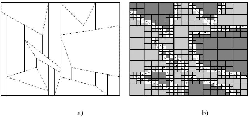
There are a number of environment representations based on C-space. The most common representations are explained in the following sections, based on the scenario represented by the C-space as depicted in Figure 2.1 (b).

Figure 2.1: A scenario represented in (a) original form (b) configuration space. The darker rectangles in (a) are those with actual dimensions while in (b) are those enlarged according to the size of vehicle A. The white areas denote the free space.

Start

Goal

A

Start

Goal

2.4 Cell Decomposition (CD)

The cell decomposition method uses non overlapping cells to represent the free-space (Cf) connectivity. The decomposition can be exact or approximate. An exact

decomposition divides Cf exactly [8]. An approximation scheme Kambhampati

discretizes Cf with cells. It decomposes the free space recursively, stopping when a

cell is entirely in Cf or entirely inside an obstacle. Otherwise, the cell is further

divided. Because of memory and time constraints, the recursive process stops when a certain degree of accuracy has been reached. The cell decomposition method,

although simple to implement, seldom yields high-quality paths. The exact cell decomposition technique is faster than the approximate one, but the path obtained is not optimal. The approximate cell decomposition can yield near-optimal paths by increasing the grid resolution, but the computation time will increase drastically. There is also the known problem of digitization bias associated with using a grid. This stems from the fact that while searching for the shortest path in a grid, the grid distance is measured and not the Euclidean distance.A visualization of this approach is shown in Figure 2.2.

a) b)

Figure 2.2: a) Exact cell decomposition, Cfree exactly decomposed into trapezoids;

9

2.5 Roadmap (RM)

The roadmap method is a popular approach to motion planning. Roadmap (RM) represents the C-space of obstacles and vehicle with edges and nodes by constructing graphs or maps. A graph G is made of a set of vertices or nodes V(G) as well as a set of edges/lines E(G). E(G) is an unordered pair of distinct vertices of G [40]. RM typically takes several steps to build a graph or map for path planning purpose, starting with establishment of nodes’ connections with edges within the free C-space

area. Next the starting point pstart and target point ptarget of the vehicle are combined to the network to complete the graph or map. A collision-free path through a series of line segments is then searched from the pstart to ptarget [41] using graph search

algorithm. Roadmaps overweigh the cell decompositions method in the number of nodes as path planner needs to search through (in cell decomposition method) in order to find a path.

2.5.1 Voronoi Diagram

as an input parameter and produce a path that would be shortest while satisfying the minimum clearance requirement. The shortest path problem on its own can be viewed as only a special case when we set the clearance required to zero.

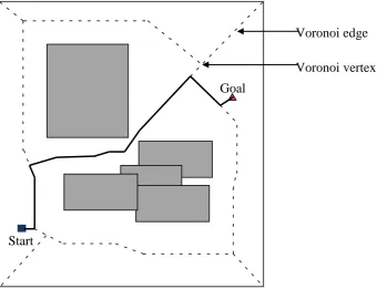
The Voronoi diagram of the configuration space is the set of collision-free configurations, whose minimal distance to Cobst is achieved with atleast two points on

the boundary of Cobst [14].

v= {q∈Cfree|d= _∈ , ∃q’, q”∈Cobstq’ ≠q”, d = dist(q,q’) = dist(q, q”)}

(2.1)

As can be seen from the example shown in Figure 2.3, if the agent moves along the Voronoi diagram, it keeps a maximum distance to all C-obstacles.

Figure 2.3: A Voronoi diagram. The dashed lines are the set of points equidistant to obstacles. The path is shown in solid darker lines.

Voronoi edge

Voronoi vertex

Start

11

2.5.2 Probabilistic Roadmap

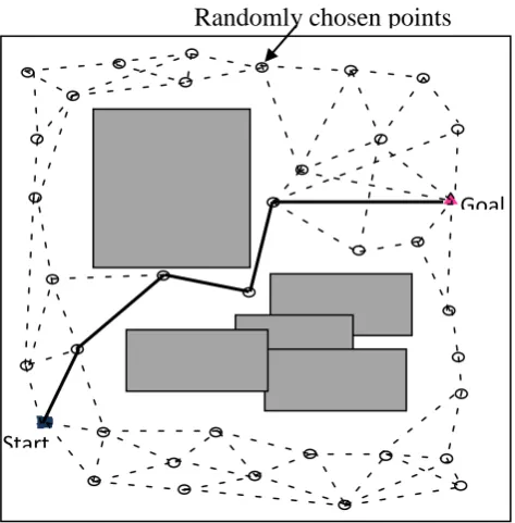
Probabilistic Roadmap (PRM) is a popular method for path planning as it is easy to apply. It makes path planning in large or high-dimensional spaces tractable and provides a good approximation of the connectivity of the configuration space area Qfree. This method consists of two phases i.e. learning phase and query phase.

Learning phase constructs a graph G whose nodes are on the free Qfree and the edges

connect the nodes without intersecting any obstacle.

On the other hand, query phase connects the starting point pstart and target point ptarget to G. A search algorithm is then used to find a path from pstart to ptarget. Figure 2.4 shows an example of PRM used in path planning. A path connecting the starting point and target point is illustrated in solid black line. However, the

construction of roadmap is computationally expensive as it might sample thousands of nodes to ensure a path exists. Furthermore the generated path often has poor quality as a result of the randomness inherent in the graph that represents the Qfree

connectivity. This method may also be incomplete i.e. do not find a path between two locations although there exist a path connecting them, in the present of narrow passage. In addition, there is no way to know whether a path exists as long as no path has been found [42].

Figure 2.4: A PRM which nodes are chosen randomly Randomly chosen points

Start

2.5.3 Rapidly-exploring Randomise Tree

Rapidly-exploring Randomise Tree (RRT) which is introduced by [43] is a variation of PRM. RRT begins at both starting point pstart and target point ptarget, and randomly expands tree for the whole configuration space. The idea is to incrementally construct a roadmap which expands the connected paths toward the areas which have not been covered yet. In order to construct a map using RRT, consider a tree, T which is one of Tps and Tpt originated at Pstart and Ptarget, respectively. T is then extended incrementally by adding a random node, qr in Qfree in uniform manner at

each iteration by sampling a nearest node qn to qr. The T tries to connect qr to qn subject to kinematic constraints which result in a new node qw. The new edge connecting qn and qr is included in the set of edges of T [44]. Readers are referred to [43] for a further explanation of RRT. One example of multiple RRTs which T started from both pstart and ptarget is shown in Figure 2.5 where the planned path is shown in solid dark lines. There are several advantages of RRT including relatively simple, suitable for finding a path for vehicle with dynamic and physical constraints, the expansion of RRT is heavily biased toward unexplored areas of C-space and it is minimal in terms of the number of edges, to name just a few. However, the resulted path from RRT is always not optimal.

Figure 2.5: Path Planning using multiple RRTs

Start

13

2.6 Potential Field

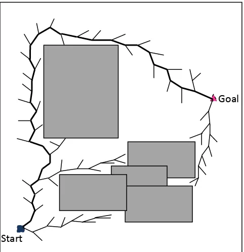
The idea behind the potential field (PF)method is to assign afunction similar to theelectrostaticpotential to each obstacleand then derive the topological structure of the free space in theform of minimum potential valleys. The robot is pulled

towardthe goal configuration as it generates a strong attractive force. Incontrast, the obstacles generate a repulsive force to keep therobot from colliding with them. The path from the start to thegoal can be found by following the direction of the

steepestdescent of the potential toward the goal [11]. The strength of thisapproach is that path planning can be done in real time by consideringonly the obstacles close to the robot. Information onthe locations of all obstacles is not required beforehand. However,as only local properties are used in planning, the robot mayget stuck at localminima and never reach the goal. The potential field approach is illustrated in Figure 2.6.

Figure 2.6 The potential field approach

2.7 Bezier Curve

control points, P0, P1, ..., Pn. The generalised Bezier curve, CB(l) is defined as follows [109]:

(2.2)

where ∈ and are Bernstein basis polynomials.

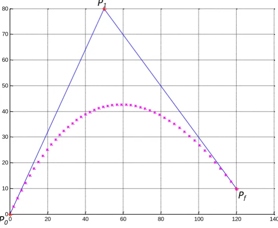
In order to illustrate the curves generated by Bezier curve technique, consider two piece-wise paths which are shown in blue in Figures 2.7 and 2.8 with one and two waypoints, respectively. The Bezier curves (dotted magenta lines) are then generated by second and third orders as shown in Figure 2.7 and Figure 2.8, respectively.

Figure 2.7: A 2nd order (quadratic) Bezier curve with three control points

0 20 40 60 80 100 120 140

0 10 20 30 40 50 60 70 80

P0

P1

15

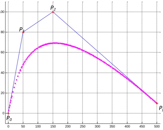
Figure 2.8: A 3rd order (cubic) Bezier curve with four control points

Both Figures 2.7 and 2.8 clearly show that the curves pass through the first, P0 and last control points, Pf and pulled in the direction of the middle points. The

curve is also tangent to the P0P1 line segment at the start and the last line segment, Pf

-1Pf at the end. These characteristics present for any order of Bezier curve and are

advantageous for path smoothing as these will make the robot to gradually leave the first line segment and go to the last line segment smoothly.

2.8 Comparison of the Method

Based on Voronoi diagram method for path planning, firstly, there needs known static obstacles which construct the Voronoi diagram, then obtained the shortest path by optimal search algorithm. The Voronoi diagram can generate the origin robot path points, and reduce the path search time.

The advantage of using a Voronoi diagram as a roadmap over a visibility graph is that the Voronoi diagram can be constructed in just O(nlogn) time whereas even the fastest known algorithm for constructing visibility graph [9] can take O(n2) time in worst case when the visibility graph has O(n2) edges. Since a Voronoi

0 50 100 150 200 250 300 350 400 450 500

0 20 40 60 80

100 P2

P0

P1

diagram has O(n) edges, querying for a path in a Voronoi diagram based roadmap is also much faster than querying in a visibility graph.

However, as mentioned before, the quality of path obtained directly from the Voronoi diagram may not be good and is usually far from optimal. So in recent years, improving the quality of the path has been an active area of research. In [15], the authors combine the Voronoi diagram, visibility graph and potential field

approaches to path planning into a single algorithm to obtain a tradeoff between safest and shortest paths. The algorithm is fairly complicated and although the path length is shorter than those obtained from potential field method or Voronoi diagram, it is still not optimal. The path exhibits bumps and rudimentary turns and is not smooth. Another recent work on reducing the length of the path obtained from a Voronoi diagram can be observed in [7]. The method involves constructing polygons at the vertices in the roadmap where more than two Voronoi edges meet. The path is smoother and shorter than that obtained directly from the Voronoi diagram but there has been no attempt to reach optimality. In [20], the authors create a new diagram called the V V(c) diagram (the Visibility-Voronoi diagram for clearance c). It is similar to this project which is to obtain an optimal path for a specified clearance value. The diagram evolves from the visibility graph to the Voronoi diagram as the value of c increases.

Unfortunately, as the method is visibility based, the processing time is O(n2logn) which renders it impractical for large spatial datasets. Apart from roadmap based techniques, the potential field approach [10],[19] and cell decomposition method [12], [5] are two popular path planning approaches. The potential field approach is simple but has several potential problems, such as being trapped in local minima or failure to pass through small openings [13]. In particular, the robot may get stuck at a local minimum. The paths obtained by cell

17

2.9 Search Algorithm

At its core, the search algorithm or a path finding method searches a graph by starting at one vertex and exploring adjacent nodes until the destination node a reached, generally with the intent of finding the shortest route. To find a path between two nodes in a graph and to find the shortest path problem this algorithm will be use. During the search, each configuration is allowed to have only one parent, otherwise, the robot keep moving in cycle [33].

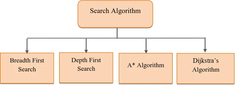
This section presents a brief review of basic graph searching principles for edge detection applications. A graph consist a set of points called nodes and a set of links that determine how the nodes can be connected [34]. The connections between start node and end node are defined as set of links. There are several search method develop here are several search method develop in artificial intelligence such as Breadth First, Depth First, A* and Dijkstra’s Algorithm [33] as shown in Figure 2.9.

Figure 2.9: Classifications of the Search Algorithms Search Algorithm

Dijkstra’s Algorithm A* Algorithm

Breadth First Search

2.9.1 Breadth-first Search

In graph theory, breadth-first search (BFS) is a graph search algorithm that begins at the root node and explores all the neighboring nodes. Then for each of those nearest nodes, it explores their unexplored neighbor nodes, and so on, until it finds the goal [36]. The theory support in [37] that states the search starts at the root and then visits all of the children of the root first. Next, the search then visits all of the grandchildren, and so forth. The belief here is that the target node is near the root, so this search would require less time. BFS considers each of the nodes that are the same link length from the start node before going onto second stages [37]. This method seem like Dijkstra's algorithm, it is to find the shortest paths, but with every edge having the same length. This algorithm more simple and does no need any data structures.

Breadth-First searches keep all the possible paths to be keeping in memory at once, evaluating them simultaneously. These algorithms will always find the shortest path on its first run and are more appropriate when there are a small number of solutions, which take a relatively short number of steps [36]. However, it will waste time considering irrelevant cycles. These operations will typically require more time and must be count as part of the algorithm’s complexity in practice [39].

Step 1: Explore paths [A B]

(Goal not found) [A C] [A D]

Step 2: Explore paths [A B E](Dead end) (Goal not found) [A B F](Dead end)

[A C G]

[A D H](Dead end) Step 1: Explore paths [A C G END]

Path is success!

Figure 2.10: Breadth First Search. (Adapted from [36]). The gray line is visited line while the red line is the path.

A

C D

B

F E

END

G _H

START

19

2.9.2 Depth-first search

Depth-first search (DFS) algorithm searches a path by moving towards the ending point as rapidly as possible and will continue moving to another path until it finds a dead end. It's means, this algorithm doesn't explore every avenue simultaneously, but chooses the avenue which gets it closer to the goal, and only explores that avenue until it is proven successful or unsuccessful. It searches one path to a leaf before following any other path [36]. DFS algorithm work best for problems where there are many possible solutions, and only one of them is required. At this task, it will operate much faster than a Breadth-First system.

Depth-First search can only find the minimum length path by searching through the whole graph, rather than stopping at the first solution. It is the method of choice when there is a known short length to paths but there are a large number of alternatives to sort. In term of the memory space, this algorithm requirement less than breadth because only linear with respect to the search graph [36]. However, this algorithm explores as far as possible along each branch before backtracking. Even a finite graph can generate an infinite tree. This method is also call brushfire, since it resembles the way fire progresses in dry grassland. This method can find the shortest path, but it examines a large part of the space. It is obvious that both of these are not very efficient [33].

Step 1: Explore paths [A B]

Step 2: Explore paths [A B E] (Dead end) [A B F] (Dead end)

Step 3: Explore paths [A C]

Step 4: Explore paths [A C G]

Step 5: Explore paths [A C G END]

Path is success!

Figure 2.11: Depth first search. (Adapted from [36]) The gray line is visited line while the red line is the path.

A

C D

B

F E

END

G _H

START

2.9.3 A* Algorithm

The A* algorithm is one of the search algorithms which is quite popular among programmer. This algorithm provides a solution that efficiently enough for optimal path finding process [35]. This algorithm used when a solution with a minimum cost desired and there must underestimate of the cost from the current configuration to the goal. The better the cost-to-go approximates the actual cost, the more A* can prune out partially generated paths, making it more efficiently [33, 37].

The advantages of this algorithm are it is complete provided that the node does not underestimate how close the node is to goal and it is optimal in that it will provide the fastest search of any other shortest path algorithm which uses the same heuristic [36]. Although this algorithm can find a path in a relatively short time but in fact the path are not optimal and smooth. It is also required a lot of memory.

Step 1:Explore paths O {O,A} f=1+5=6 , {O,B} f= 2+6=8 Step 2:Explore paths A

{O,B} f= 2+6=8

{O,A,F} f= (1+4)+5=10 {O,A,E} f= (1+7)+8=16 Step 3:Explore paths B {O,A,F} f= (1+4)+5=10 {O,B,C} f= (2+7)+4=13 {O,A,E} f= (1+7)+8=16 {O,B,D} f= (2+1)+15=18 Step 3:Explore paths END

{O,A,F,END}is the best path(cost 7)

Figure 2.12: A* Algorithm. (Adapted from [38]). The gray line is visited line while the red line is the path.

6 3

START

5 3

2

5

8 ₄ 15

0

1

END

A B

G _J

E F

H I

C D

21

2.9.4 Dijkstra’s Algorithm

Dijkstra’s shortest part algorithm for graph is useful for path planning [33]. Dijkstra’s algorithm is the most efficient when it is searching for the shortest path

between two nodes [33,37]. Starting from a goal node, it finds the nodes connected to the goal, puts them in a queue, and assigns each of them the cost to goal, which is the weight of the edge connecting it to the goal.

Dijkstra’s algorithm is able to find a shortest path that connects a starting and

target points. This algorithm does much more searching than is necessary, but is guaranteed to find the shortest path [36]. Although Dijkstra's algorithm is fast, it suffers from its inability to deal with negative edge weights [38]. This algorithm is often used in routing and as a subroutine in other graph algorithms. It also can be used for finding costs of shortest paths from a single vertex to a single destination vertex by stopping the algorithm once the shortest path to the destination vertex has been determined [34]. Figure 2.13 below illustrates the Dijkstra’s Algorithm.

Step 1: Explore paths [OAE END] (7)

Step 2: Explore paths [OCK END] (8)

Step 3: Explore paths [OBI END] (5)

Step 4: Explore paths [OBG END] (4)

Path is success!

Figure 2.13 Dijkstra’s Algorithm. The green line is visited line while the red line is the path.

C L

START

A D

B

F

E _J K

2.10 Car-Like Robot Model

Firstly, a ‘standard model’ for the vehicle and its workspace is introduced. This is the

representation of the car-like robot used throughout the development of the path planning, obstacle avoidance and tracking systems. The model given below is based upon those described in [14] and [31].

Let A be a car-like robot, capable of only forward motion, modeled as a rigid rectangular body moving on a planar (two-dimensional) workspace, W ≡ R2, that is free of obstacles. A is supported by four wheels making point contact with the ground, while it has two fixed rear wheels and two directional (steerable) front wheels. The wheelbase (distance between front and rear wheels) is denoted by L. Λ is the configuration of A within W defined by the following quartet, (x, y, θ, κ) where (x, y) are the coordinates of the rear axle midpoint. θ(the vehicle’s orientation) is the angle between the x-axis and the main axis of the vehicle (−π _ θ _ π)5. Steering angle is denoted as φ and determines the instantaneous centre of rotation Ω of the robot. The position of Ω determines the instantaneous radius of curvature ρ of the vehicle’s path, given by L/ tan φ [14]. The instantaneous curvature κ of the robot is

the inverse of the instantaneous radius of curvature (κ = ρ−1). Finally, the vehicle’s velocity at the centre of its rear axle is defined as V. This vehicle model is shown in Figure 2.14.

23

2.11 Previous Study on Voronoi Diagrams

This section will review several recent papers that are using Voronoi diagram method for path planning. [17] addresses the problem of on-line path following for a car working in unstructured outdoor environments. The partially known map of the environment is updated and expanded in real time by a Simultaneous Localization and Mapping (SLAM) algorithm. This information is used to implement global path planning. A cost graph is initially constructed followed by a search to find the near-optimal path considering uncertainty in both vehicle location and map. Selected points in the global path are connected by continuous-curvature paths. An improved feedback linearization technique is presented to guide the car along the defined path.

[24] gives an algorithm for generating the Voronoi diagram from the points set on a cylinder by modification process to improve the efficiency of the weld testing for acylindrical oilcan performed by the wall-climbing robot. Based on this algorithm the paper also provides a method about thedesign of cylindrical tank wallboards and the weld testing pathplanning from Delaunay Triangulation. A software simulationplatform is also developed. The simulation results show that themethod is effective to the stand cylindrical tank design and thewall-climbing robot weld testing path planning.

A new motion planning technique, which is built on the generalized Voronoi diagram, for a robot with kinematic or dynamic constraints is proposed in [18]. The generalized Voronoi diagram serves this task effectively as it maintains the largest (the safest) possible distance from surrounding obstacles. Moreover, a novel approximation geometric algorithm, which embodies a trade-off between the

efficiency of computation, implementation difficulty, and robustness, for computing this diagram is presented.

[21] present a simulated annealing (SA) based algorithm for robot path planning. The kernel of the SA engine is based on Voronoi diagram and composite Bezier curve to obtain the shortest smooth path under given kinematic constraints. In the algorithm, a Voronoi diagram is constructed according to the global environment. The piecewise linear path in the Voronoi diagram which keeps away from the

obstacles is obtained by performing Dijkstra’s shortest path algorithm. The control

composite Bezier curve path while satisfying givenkinematic constraints. Experimental results on two mapscontaining sharp turns demonstrate the effectiveness of theproposed SA-based smooth path planning algorithm.

Meanwhile [16] presents a new sensor based global Path Planner which operates in two steps. In the first step the safest areas in the environment are

REFERENCES

[1] Cang, YE. (2005). A Method For Mobile Robot Obstacle Negotiation. International Journal of Intelligent Control and Systems, 10(3), 188-200.

[2] M. Kruusmaa, J. Willemson. (2003). Covering the Path Space: A Casebase Analysis for Mobile Robot Path Planning. Knowledge-Based Systems, 16, 235-242.

[3] M. Ruehl, H. Roth. (2005). Robot Motion Planning by Approximation of Obstacles in Configuration Space. 16th IFAC World Congress, 6.

[4] Y.K. Hwang, N. Ahuja. (1992). Gross Motion Planning - A Survey. ACM Computing Survey, 24(3), 219-291.

[5] Chen, D.Z., Szczerba, R.J., Uhran, Jr., J.J. (1997). A Framed-Quadtree Approach for Determining Euclidean Shortest Paths in a 2-D Environment. IEEE

Transactions on robotics and automation, 13(5).

[6] de Berg, Mark, Marc van Kreveld, Mark Overmars, Otfried Schwartzkopf. (1997). Computational Geometry: Algorithms and Applications. Springer.

[7] Dong-Hoon, Y., Suk-Kyo, H. (2007). A roadmap construction algorithm for mobile robotpath planning using skeleton maps. Advanced Robotics, 21(1-2), 51-63.

[8] F. Avnaim, J. D. Boissonnat, B. Faverjon. (1988). A practical exact motion planning algorithm for polygonal objects amidst polygonal obstacles. Proc.IEEE Int. Conf. Robotics and Automation, 3, 1656–1661.

[9] Ghosh, S.K., Mount, D.M. (1991). An output-sensitive algorithm for computing visibility graphs. SIAM J. Computing, 20.

[10] Hussien, B. (1989). Robot Path Planning and Obstacle Avoidance by Means of Potential Function Method. Ph.D Dissertation. University of Missouri-Columbia.

[11] J. Borenstein, Y. Koren. (1998). Real-time obstacle avoidance for fast mobile robot. IEEE Trans. Syst., Cybern, 19(5), 1179-1187.

[13] Koren, Y. B. (1991). Potential Field Methods and Their Inherent Limitations for Mobile Robot Navigation. IEEE Conference on Robotics and Automation, (pp. 1398–1404).

[14] Latombe, J.C. (1991). Robot Motion Planning. USA: Kluwer Academic Publishers.

[15] Masehian, E., Amin-Naseri, M.R. (2004). A voronoi diagram-visibility graph-potential field compound algorithm for robot path planning. Journal of Robotic System, 21(6).

[16] Santiago Garrido, Luis Moreno, Dolores Blanco, Piotr Jurewicz. (2011). Path Planning for Mobile Robot Navigation using Voronoi Diagram and Fast Marching. International Journal of Robotics and Automation, 2(1), 42-64.

[17] Shahram Rezaei, Jose Guivant, Eduardo M. Nebot. (2003). Car-Like Robot Path Following In Large Unstructured Environments.

[18] Svec, P. (2008). Kinodynamic Robot Motion Planning Based On The Generalised Voronoi Diagram. Engineering Mechanics, 15, 139-150.

[19] Warren, C. (1989). Global Path Planning Using Artificial Potential Fields. IEEE Conference on Robotics and Automation, (pp. 316–321).

[20] Wein, R., Van den Berg, J.P., Halperin, D. (2005). The Visibility-Voronoi complex and its applications. 21st Annual Symposium on Computational geometry, (pp. 63-72).

[21] Yi-Ju Ho, Jing-Sin Liu. (2010). Simulated Annealing based Algorithm for Smooth Robot Path Planning with Different Kinematic Constraints. 1277-1281.

[22] J. Cortes, F. Bullo. (2005). Coordination and geometric optimization via distributed dynamical systems. SIAM J. Control Optim., 44(5), 1543–1574.

[23] Aurenhammer, F. (1991). Voronoi diagrams—A survey of a fundamental geometric data structure. ACM Computing Surveys, 23(3).

[24] Zhuang Fu, Zhao Yan-zheng, Qian Zhi-yuan, Cao Qi-xin. (2006). Wall-climbing Robot Path Planning for Testing Cylindrical Oilcan Weld Based on Voronoi Diagram. IEEE/RSJ International Conference on Intelligent Robots and Systems, (pp. 2749-2753).

66

[26] Guibas, L.J., Knuth, D.E., Sharir, M. (1992). Randomized incremental construction of Delaunay and Voronoi diagrams. Algorithmica, 7, 381–413.

[27] M. L. Gavrilova, J. G. Rokne. (2003). Collision detection optimization in a multi-particle system. Int. J. Comput. Geometry Appl., 13(4), 279–301.

[28] P. Bhattacharya, M. L. Gavrilova. (2006). CRYSTAL—A new densitybased fast and efficient clustering algorithm. 3rd Int. Symp. Voronoi Diagrams in Science and Engineering, (pp. 102–111).

[29] R. Apu, M. L. Gavrilova. (2006). Battle swarm: An evolutionary approach to complex swarm intelligence. 9th Int. Conf. Computer Graphics and Artificial Intelligence, (pp. 139–150).

[30] R. Graham, J. Cortes. (2009). Asymptotic optimality of multicenter Voronoi configurations for random field estimation. IEEE Trans. Automat. Contr.

[31] Scheuer, A., Fraichard, T. (1997). Continuous-Curvature Path Planning for Car-Like Vehicles. IEEE/RSJ Int. Conf. on Intelligent Robots and Systems.

[32] K. G. Joll, R. S. Kumar and R. Vijayakumar. (2009). A Bezier curve based path planning in a multi-agent robot soccer system without violating the acceleration limits. Elsevier Journal of Robotics and Autonomous Systems, 57(2009), pp 23– 33.

[33] Yong K.H and Ahuja.N, (1992), "Gross motion planning—a survey," ACM Computing Surveys, vol. 24, pp. 219 - 291.

[34] M. L. Wager.(2000), "Making Roadmaps Using Voronoi Diagrams" [Online]. Available:http://www.cs.cmu.edu/~biorobotics/papers/sbp_papers/integrated4/mi cha_voronoi.pdf.

[35] Khuswendi.T, Hindersah.H,and Adiprawita.W, (2011), "UAV Path Planning Using Potential Field and Modified Receding Horizon A* 3D Algorithm," in International Conference on Electrical Engineering and Informatics, Bandung.

[37] Choset.H and all, (2007), "Principles of Robot Motion: Theory,Algortihms and implementations", [Online]. Available: http://www.cs.cmu.edu/~ biorobotics/book/booboo_book.pdf, Retrieved on 1 April 2011.

[38] Graph Theory: Shortest Path. The shortest path problem [Online]. Available:

http://www.cs.cornell.edu/~wdtseng/icpc/notes/graph_part2.pdf, Retrieved on

2nd Apr 2012.

[39] Omar.R and Gu.W.G, (2009), "Visibility Line Based Methods for UAV Path Planning," in ICROS-SICE International Joint Conference 2009, Fukuoka, p. 3176.

[40] C. Godsil and G. Royle. (2001). “Algebraic Graph Theory”. Springer.

[41] R. Siegwart and I. R. Nourbakhsh. (2004). “Introduction to autonomous mobile robots”. Bradford Company, Scituate, MA, USA.

[42] J. L. Latombe. (1999). “Motion planning: A journey of robots, molecules, digital actors, and other artefacts”. In International Journal of Robotics Research, 18(11), pp 1119-1128.

[43] S. M. LaValle. (1998). “Rapidly-exploring random trees: A new tool for path planning”. TR 98-11, Computer Science Dept., Iowa State University.

[44] H. Choset, G. Kantor, W. Burgard, L. Kavraki and S. Thrun. (2005). “Principles of robot motion: Theory, algorithms, and implementations”. The MIT Press.