Comparisons of Individual and Group Replacement Policies for a Two machine Series System

Comparisons of Individual and Group Replacement

Policies for a Two-machine Series System

Wen Liang Chang

1,*

_{, Mei Wei Wang}

2

1_{General Education of Holistic Education Center, Cardinal Tien Junior College of Healthcare & Management, Taiwan} 2_{Department of Industrial Management, National Taiwan University of Science and Technology, Taiwan}

Copyright©2016 by authors, all rights reserved. Authors agree that this article remains permanently open access under the terms of the Creative Commons Attribution License 4.0 International License

Abstract

This paper studies the comparisons of individual and group replacement policies for a two-machine series system. Suppose that manufacturer’s production system which consists of two machines in series. For two machines, when any machine fails within the operating time, minimal repair is performed for machines by the manufacturer. Due to the inevitable deterioration of the machine, the machine may fail more frequently as its age or usage increases. Therefore, an appropriate preventive replacement (PR) of the machine may be suitable for reducing the number of failures and maintains the operation of the machine normally. When a PR action is performed, it incurs a replacement cost and a downtime cost. Hence, when the replacement cost is high, it might be worthwhile replacing both machines at the same time (called group replacement policy; GRP) instead of replacing them separately (called individual replacement policy; IRP). Under these maintenance policies, the maintenance cost rate models of individual and group replacement for a series system is derived and further, optimal preventive replacement time is obtained such that the expected total cost rate is minimized. Finally, some numerical examples are given to illustrate the influences of individual and group replacement policies to the expected total cost rate.

Keywords

Individual Replacement, Group Replacement, Two-machine, Series System

1. Introduction

In the production process, it is an important item whether production system is normal operation. In general, a production system involves multiple subsystems (or machines). To maintain production system normal operation, a suitable maintenance policy for subsystems (or machines) should be planned and performed. Usually, maintenance policy can be classified into corrective maintenance (e.g. minimal repair, imperfect repair and

perfect repair) and replacement. For the failed equipment, minimal repair is often adopted to correct failed equipment back to its normal operation status. After minimal repair, the equipment is normal operation, but the failure rate function remains unchanged. Nakagawa and Kowada [1] defined a minimal repair in the failure rate of devices and proposed the replacement model of system. The replacement model where a system is replaced at a fixed time or at nth failure is considered and further, the optimal replacement policies are obtained. Nakagawa [2] summarized four models of modified periodic replacement with minimal repair at failures when the replacement time is pre-specified. If a unit fails just before the replacement time, then three replacement policies for a unit are considered: i) a unit remains as it is until the replacement time comes, ii) a unit is replaced by one of spares, iii) a unit is replaced by a new unit. In addition, if a unit fails well before replacement time then the unit is replaced at failure or at a fixed time. Under those policies, the expected cost of each model is constructed and the optimal replacement policy is obtained. Boland and Proschan [3] proposed two cost models with minimal repair and periodic replacement policies: A) the total expected cost of repair and replacement over a fixed time horizon and B) the total expected cost per unit time over an infinite time horizon. For two models, the optimal replacement time is obtained and numerical examples are given to illustrate the impacts of replacement policy for the cost models. Various maintenance models involving minimal repair can be found in the literatures (Phelps [4], Sheu [5], Jaturonnatee et al. [6], Chien and Sheu [7], Laggoune et al. [8], Sheu et al. [9], Li and Peng [10]).

illustrate the impact of a product warranty on the optimal periodic replacement policy. Sheu [12] investigated the impacts of the block replacement policy a system subject to shocks. Consider that an operating system is preventively replaced by new ones at a fixed time and the optimal policy is discussed. Further, various special cases are considered and numerical examples are given and illustrated. In addition, FR is performed when the product fails. Cheng and Li [13] studied a deteriorating repairable system with two-types of failure states and used a replacement policy N

based on the failure number of the system to construct average cost rate of the system. Then, an optimal replacement policy N* _{is obtained such that the average cost} rate of the system is minimized. Qian et al. [14] considered replacement and minimal repair polices for an extended cumulative damage model with maintenance at each shock. Suppose that a system undergoes minimal repair at each shock when the total damage exceeds a failure level, and is replaced at time T* _{or at failure N}* _{whichever occurs first.} The expected cost rate is constructed and the optimal T* _and

N* _{is obtained which minimizes the expected cost. For the} product, various replacement policies of the product can be found in the literatures (Moghaddam and Usher [15], Zhang and Wang [16], Sheu and Zhang [17], Vu et al. [18]).

In this paper, the individual and group replacement cost models of a two-machine series system is derived and optimal individual and group replacement time are obtained. Further, the comparisons of individual and group replacement policies for a series system are illustrated through numerical examples. The outline of this paper is described as follows. Two model formulations are derived in Section 2. The optimal individual and group replacement policies are obtained in Section 3. In Section 4, the comparisons of individual and group replacement policies are illustrated through numerical examples. Finally, some conclusions are drawn in the last section.

2. Model Formulation

Suppose that Manufacturer’s production system consists of two machines (Mi, i=1, 2) using series connection method. The probability density distribution, failure rate, and cumulative failure rate of the machines Mi are fi(t), hi(t) and Hi(t), i=1, 2, respectively. The cumulative failure rate is

du

u

h

t

H

i

(

)

=

∫

₀t i

(

)

. Manufacturer plans to perform

preventive replacement for the machines at a pre-specified time to maintain system normal operation. The individual and group replacement for the machines Mi are performed at a pre-specified time Ti, i=1, 2 and Tg, respectively.

Under IRP, when the age of the machine Mi reaches a pre-specified time Ti, a replacement action for the machine is performed and incurs a replacement cost Cri, i=1, 2 and a downtime cost Cdr1+Cdr2. Hence, the expected total replacement cost of the machine Mi is Cri+Cdr1+Cdr2, i=1, 2. Before replacement time Ti, any machines Mi fails, minimal

repair is performed and incurs a repair cost Cmi, i=1, 2and a downtime cost Cdm1+Cdm2. Since the failure of the machine

Mi is corrected by the minimal repair, the failure process of the machine is a non-homogeneous Poisson process with intensity function hi(t), i=1, 2. Therefore, within the pre-specified individual replacement time Ti, the expected total repair cost of the machines Mi is (Cmi+Cdm1+Cdm2)Hi(Ti), i=1, 2. The combination of expected total replacement and repair costs, within individual replacement time Ti, i=1, 2, the expected total cost rate of the system can be obtained as follows.

∑

=

+

+

+

+

+

=

=

2

1

2 1 2

1 2 1

)

(

)

(

)]

,

(

[

i i

dr dr ri i i dm dm mi

T

C

C

C

T

H

C

C

C

T

T

C

E

. (1)

Under GRP, when the age of the machine Mi reaches a pre-specified time Tg, two machines are replaced simultaneously and incurs a replacement cost Cr1+Cr2 and a downtime cost Cdr1+Cdr2. Hence, the expected total replacement cost is Cr1+Cr2+Cdr1+Cdr2. Within group replacement time Tg, the expected total repair cost of GRP is the same as IRP. Hence, the expected total repair cost is (Cmi+Cdm1+Cdm2)Hi(Tg), i=1, 2. The combination of expected total replacement and repair costs, within group replacement time Tg, the expected total cost rate of the system can be obtained as follows.

g

dr dr r r

i mi dm dm i g

g

T

C C C C T H C C C T C E

2 1 2 1 2

1 1 2

)] ( ) [(

)] ( [

+ + + + +

+ =

=

∑

=

.

(2) The objective of this paper is to find the optimal individual replacement time ( *

1

T

, * 2

T

) and group replacement time *

g

T

such that the expected total cost rate

E[C(T1,T2)] and E[C(Tg)] in Eqs. (1) and (2) is minimized, respectively.

3. Optimal Replacement Policy

Based on the objective functions (1) and (2), the optimal individual and replacement policies are derived as follows.

3.1. Individual Replacement

To investigate the optimal individual replacement time Ti, we take the first partial derivative of Eq. (1) with respect to

Ti, i=1, 2 and then the result is

2

,1

,

)

(

)

(

)]

,

(

[

2

2 1 2

1

₌

−

+

+

₌

∂

∂

i

T

C

C

C

T

K

T

T

T

C

E

i

dr dr ri i i

i

Observing Ki(Ti), i=1, 2, the following property holds. Property 1. If

_h

_i

′

(

_t

)

>

0

,

_i

=

1

,

2

,

∀

_t

>

0

, then we have Ki(Ti) is a strictly increasing with Ti,

lim

(

)

0

0

=

→ i i

Ti

K

T

,

and

lim

(

)

>

0

∞ → i i

Ti

K

T

, i=1, 2.

Proof. If

_h

_i

′

(

_t

)

>

0

,

_i

=

1

,

2

,

∀

_t

>

0

, then we have

dKi(Ti)/dTi > 0. This implies that Ki(Ti) is a strictly increasing function of Ti and

lim

(

)

0

0

=

→ i i

Ti

K

T

, i=1, 2. Since

Ki(Ti) is a strictly increasing function, then

lim

(

)

>

0

→∞ i i

Ti

K

T

,

i=1, 2.

Observing Eq. (3), the following theorem holds.

Theorem 1. When

_h

_i

′

(

_t

)

>

0

,

_i

=

1

,

2

,

∀

_t

>

0

,the following results hold.

(a) If Ki(∞)<Cri+Cdr1+Cdr2, then optimal

T

i*

=

∞

, i=1,

2.

(b) If Ki(∞)≥Cri+Cdr1+Cdr2, then there exists a unique

solution *_∈[ ,0_∞)

i

T such that

0 ) (

)

( i* − ri+ dr1+ dr2 =

i T C C C

K , i_{=1, 2.}

Proof. When

_h

_i

′

(

_t

)

>

0

,

_i

=

1

,

2

,

∀

_t

>

0

, hi(t) is a strictly increasing function and the following results hold.

(a) If Ki(∞)<Cri+Cdr1+Cdr2, then ∂E[C(T1,T2)]/∂Ti<0, i=1, 2. This implies that E[C(T1,T2)] is a decreasing function of

Ti, i=1, 2. Therefore, the optimal

T

i*

=

∞

, i=1, 2.

(b) If Ki(∞)≥Cri+Cdr1+Cdr2, then ∂E[C(T1,T2)]/∂Ti≥ 0,

i=1,2. From the results of property 1, Ki(Ti) is a strictly increasing function. Substituting Ti=0 into Ki(Ti),

Ki(0)=0<Cri+Cdr1+Cdr2, i=1, 2 is obtained. Therefore,

∂E[C(T1,T2)]/∂Ti changes its sign exactly once from negative to positive in the interval [0,∞) and there exists a unique *

_∈

[

,0

_∞

)

i

T

such that

∂

E

[

C

(

T

1

,

T

2

)]

/

∂

T

i_Ti=Ti*

=

0

,

i_{=1, 2, that is,}

(

*

)

i i

T

K

−(Cri+Cdr1+Cdr2)=0, i=1, 2. Since Ki( *

i

T

)=(Cmi+Cdm1+Cdm2)[

T

i*hi(

T

i*)−Hi(

T

i*)] in

Eq. (3) and

(

*

)

i i

T

K

−(Cri+Cdr1+Cdr2)=0, the following equation can be obtained.

(Cmi+Cdm1+Cdm2)Hi(

T

i*)+Cri+Cdr1+Cdr2=(Cmi+Cdm1+Cdm2) *

i

T

hi( *

i

T

), i=1, 2. (4) Substituting Eq. (4) into Eq. (1), the expected total cost rate of the system can be rewritten as

∑

=

+

+

=

2

1

* 2 1 *

2 *

1

,

)]

(

)

(

)

(

[

i mi dm dm i i

T

h

C

C

C

T

T

C

E

. (5)

3.2. Group Replacement

Based on Eq. (2), taking the first derivative of Eq. (2) with respect to Tg, we have

2

2 1 2

1

)

(

)

(

)]

(

[

g

dr dr r r g

g g

T

C

C

C

C

T

K

dT

T

C

dE

−

+

+

+

=

(6)

where

∑

=

−

+

+

=

2

1

(

1 2

)[

(

)

(

)]

)

(

i mi dm dm g i g i g g

C

C

C

T

h

T

H

T

T

K

.

Observing K(Tg), the following property holds.

Property 2. If

_h

_i

′

(

_t

)

>

0

,

_i

=

1

,

2

,

∀

_t

>

0

, then we have K(Tg) is a strictly increasing,

lim

(

)

0

0

=

→ g

Tg

K

T

, and

0

)

(

lim

>

∞

→ g

Tg

K

T

.

Proof. If

h

i

′

(

t

)

>

0

,

i

=

1

,

2

,

∀

t

>

0

, then we have

dK(Tg)/dTg > 0. This implies that K(Tg) is a strictly increasing function of Tg and

lim

(

)

0

0

=

→ g

Tg

K

T

. Since K(Tg) is a strictly increasing function, then

lim

(

)

>

0

∞

→ g

Tg

K

T

. Observing Eq. (6), the following theorem holds.

Theorem 2. When

h

i

′

(

t

)

>

0

,

i

=

1

,

2

,

∀

t

>

0

, the

following results hold.

(a) If K(∞)<Cr1+Cr2+Cdr1+Cdr2, then optimal

T

g*

=

∞

.

(b) If K(∞)≥Cr1+Cr2+Cdr1+Cdr2, thenthere exists a unique

) , 0 [

*_{∈ ∞}

g

T such that

K

(

T

g*

)

−

(

C

r1

+

C

r2

+

C

dr1

+

C

dr2

)

=

0

. Proof. When

_h

_i

′

(

_t

)

>

0

,

_i

=

1

,

2

,

∀

_t

>

0

is a strictly increasing function and the following results hold.

(a) If K(∞)<Cr1+Cr2+Cdr1+Cdr2, then dE[C(Tg)]/dTg<0 in Equation (5), that is, E[C(Tg)] is a decreasing function of

Tg. Therefore, the optimal *=∞

g

T . (b) If

K(∞)≥Cr1+Cr2+Cdr1+Cdr2, then dE[C(Tg)]/dTg≥ 0 in Eq. (6). From the results of property 2, K(Tg) is a strictly increasing function. Substituting Tg=0 into K(Tg),

K(0)=0<Cr1+Cr2+Cdr1+Cdr2 is obtained. Therefore,

dE[C(Tg)]/dTg changes its sign exactly once from negative to positive in the interval [0,∞) and there exists a unique solution

T

g* such that [ ( )]/ ₌ *=0

g g T

T g g dT

T C

dE , that is,

)

(

*

g

T

K

−(Cr1+Cri2+Cdr1+Cdr2)=0. Since

∑

=

−

+

+

=

2

1

* *

* 2 1

*

₎

₍

_)[

₍

₎

₍

_)]

(

i mi dm dm g i g i g g

C

C

C

T

h

T

H

T

T

K

and

)

(

*

g

T

∑

∑

= =

+

+

=

=

+

+

+

+

+

+

+

2 1 * * 2 1 2 1 1 1 2 1 * 2 1

)

(

)

(

)

(

)

(

)

(

i mi dm dm g i g dr

dr r r

i mi dm dm i g

T

h

T

C

C

C

C

C

C

C

T

H

C

C

C

. (7)

Substituting Eq. (7) into Eq. (2), the expected total cost rate can be rewritten as

.)

(

)

(

)]

(

[

2 1 * * 2 1 *

∑

=

+

+

=

i g i g dm dm mi

g

C

C

C

T

h

T

T

C

E

(8)

Let D=

[

(

*

)]

g

T

C

E

−

[

(

,

*

)]

2 * 1

T

T

C

E

, the following

equation holds.

)].

(

)

(

)[

(

)]

(

)

(

)[

(

)

(

)

(

)

(

)

(

* 2 2 * 2 2 1 2 * 1 1 * 1 2 1 1 2 1 * 2 1 2 1 * 2 1

T

h

T

h

C

C

C

T

h

T

h

C

C

C

T

h

C

C

C

T

h

C

C

C

D

g dm dm m g dm dm m

i mi dm dm i i

i mi dm dm i g

−

+

+

+

+

−

+

+

=

=

+

+

−

−

+

+

=

∑

∑

= = (9)

From Eq. (9), we have some results for choice group replacement or individual replacement as follows.

(1) When *

g

T

>max{ * 1

T

, * 2

T

}, the individual replacement policy should be chose.

(2) When

T

g*<min{

T

1*,

T

2*}, the group replacement should be chose.

3.2. Numerical Examples

Suppose that the lifetime distribution of Machine Mi

follows a two-parameter Weibull distribution with scale parameter αi>0 and shape parameterβi>1, i=1, 2. According

to definition of a failure rate function, the failure rate function of the Weibull distribution is

1

)

(

)

(

t

₌

t

i−

h

i

α

i

β

i

α

i β , where αi>0 and βi>1, i=1, 2 and

then the expected life time is ui=(1/α_i)Γ(1+1/β_i), i=1, 2. The following parameter values are considered for the model under u1≈u2 and u1≠u2 in Tables 1 and 2.

α1=0.5, 0.15, β1=1.4, 2, 2.5, α2=0.35, β2=1.6, 2, 2.5, 3,

Cdm1=Cdm2=Cdr1=Cdr2=100, Cm1=300, Cm2=100, Cr1=700,

Cr2=800

Tables 1 and 2 show the optimal replacement time and the optimal expected total cost rate under u1≈u2 and u1≠u2 for both individual and group replacement models. For example, when β1=1.4 and β2=2.5, the optimal group replacement time is *

₌

4

g

T

and the optimal individual replacement time are

_T

₁*

₌

6

_and

_T

₂*

₌

₃

_.

₅

_{. The expected} total cost rate for both the individual and group replacement model are E[C(

_T

_g*_{)]=957.8 and E[C(} *

1

T

, * 2

T

)]=989.8.

From Tables 1 and 2, some results are obtained as follows.

1) Under the expected life time u1≈u2, when β2>2, the expected total cost rate of group replacement is lower than individual replacement.

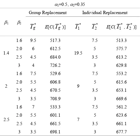
[image:4.595.315.551.199.445.2]

2) When the expected life time u1≠u2, when β2>2, the expected total cost rate of individual replacement is lower than group replacement.

Table 1.. Optimal individual and group replacement policies under u1≈u2

α1=0.5, α2=0.35

β1 β2

Group

Replacement Individual Replacement

*

g

T

_E[C( *

g

T

)]

T

1*

T

2* E[C(

T

1*,

T

2*)]

1. 4

1.6 6 862.5

6

7.5 889.9

2 5 915.0 5 952.3

2.5 4 957.8 3.5 989.8

3 3.5 982.3 3 1006.4

2

1.6 3.5 1061.6

2.5

7.5 1024.4

2 3 1070.3 5 1086.9

2.5 3 1073.5 3.5 1124.3

3 3 1076.7 3 1140.9

2. 5

1.6 2.5 1142.5

2

7.5 1051.9

2 2.5 1136.6 5 1114.4

2.5 2.5 1129.7 3.5 1151.8

3 2.5 1123.2 3 1168.4

Table 2. Optimal individual and group replacement policies under u1≠u2

α1=0.5, α2=0.35

β1 β2

Group Replacement Individual Replacement

*

g

T

E[C(

T

g*)]

T

1*

T

2* E[C(

T

1*,

T

2*)]

1.4

1.6 9.5 517.3

19.5

7.5 513.3

2.0 6 612.5 5 575.7

2.5 4.5 684.0 3.5 613.2

3 4 726.2 3 629.8

2

1.6 7.5 529.6

9

7.5 553.2

2.0 5.5 606.8 5 615.6

2.5 4.5 670.5 3.5 653.1

3 3.5 708.9 3 669.6

2.5

1.6 7 533.3

7

7.5 561.2

2.0 5.5 601.1 5 623.6

2.5 4.5 661.5 3.5 661.1

3 3.5 698.1 3 677.7

4. Conclusions

[image:4.595.313.551.467.699.2]

group replacement policies for a two-machine series system. From the results of numerical examples, we have some conclusions as follows: 1) When the failure rate of machine

M2 is a strictly increasing function, the expected total cost rate of group replacement is lower than individual replacement. 2) Under the expected life time of two machines is different, when the failure rate of machine M2 is a strictly increasing function, the expected total rate of individual replacement is lower than group replacement. Furthermore, some generalizations, such as classification replacement, multiple machines, renewing free-replacement warranty, non-renewing free-replacement warranty are extended issues for future study in this area.

REFERENCES

[1] Nakagawa, T., & Kowada, M. (1983). Analysis of a system with minimal repair and its application to replacement policy.

European Journal of Operational Research, 12, 176-182. [2] Nakagawa, T. (1981). A summary of periodic replacement

with minimal repair at failure. Journal of the Operations Research Society of Japan, 24, 213-227.

[3] Boland, P. J., & Proschan, F. (1982). Periodic replacement with increasing minimal repair costs at failure. Operations Research, 30, 1183-1189.

[4] Phelps, R. I. (1983). Optimal policy for minimal repair.

Journal of the Operational Research Society, 34, 419-424. [5] Jaturonnatee, J., Murthy, D. N. P., & Boondiskulchok, R.

(2006). Optimal preventive maintenance of leased equipment with corrective minimal repairs. European Journal of Operational Research, 174, 201–215.

[6] Sheu, S. H. (1991). Periodic replacement with minimal repair at failure and general random repair cost for a multi-unit system. Microelectronics Reliability, 31, 1019-1025.

[7] Chien, Y. H., & Sheu, S. H. (2006). Extended optimal age-replacement policy with minimal repair of a system subject to shocks. European Journal of Operational Research, 174-1, 169-181.

[8] Laggoune, R., Chateauneuf, A., & Aissani, D. (2009). Opportunistic policy for optimal preventive maintenance of a multi-component system in continuous operating units.

Computers and Chemical Engineering, 33, 1499-1510. [9] Sheu, S. H., Chang, C. C., & Chen, Y. L. (2010). A periodic

replacement model based on cumulative repair-cost limit for

system subjected to shocks. IEEE Transactions on

Reliability, 59, 374-382.

[10]Li, Y. F., & Peng, R. (2014). Availability modeling and optimization of dynamic multi-state series–parallel systems with random reconfiguration. Reliability Engineering & System Safety, 127, 47-57.

[11]Yeh, R. H., Chen, M. Y., & Lin, C. Y. (2007). Optimal periodic replacement policy for repairable products under free-repair warranty. European Journal of Operational Research, 176, 1678-1686.

[12]Sheu, S. H. (1997). Extended block replacement policy of a system subject to shocks. IEEE Transactions on Reliability,

46, 375-382.

[13]Cheng, G. Q., & Li, L. (2014). An optimal replacement policy for a degenerative system with two-types of failure states. Journal of Computational and Applied Mathematics,

261, 139-145.

[14]Qian, C., Nakamura, S., & Nakagawa, T. (2003). Replacement and minimal repair policies for a cumulative damage model with maintenance. Computers & Mathematics with Applications, 46, 1111-1118.

[15]Moghaddam, S., & Usher, S. (2011). Preventive maintenance and replacement scheduling for repairable and maintainable

systems using dynamic programming. Computers and

Industrial Engineering, 60, 654-665.

[16]Zhang, Y. L., & Wang, G. J. (2011). An extended replacement policy for a deteriorating system with multi-failure modes. Applied Mathematics and Computation,

218, 1820-1830.

[17]Sheu, S. H., & Zhang, Z. G. (2013). An optimal age replacement policy for multi-state systems. IEEE Transactions on Reliability, 62, 73-81.