BIROn - Birkbeck Institutional Research Online
Hu, W. and Fan, Y. and Xing, J. and Sun, L. and Cai, Z. and Maybank,
Stephen (2018) Deep constrained siamese hash coding network and
load-balanced locality-sensitive hashing for near duplicate image detection. IEEE
Transactions on Image Processing 27 (9), pp. 4452-4464. ISSN 1057-7149.
Downloaded from:
Usage Guidelines:
Please refer to usage guidelines at or alternatively
1
Deep Constrained Siamese Hash Coding Network and Load-Balanced
Locality-Sensitive Hashing for Near Duplicate Image Detection
Weiming Hu, Yabo Fan, and Junliang Xing
(National Laboratory of Pattern Recognition, Institute of Automation, Chinese Academy of Sciences, Beijing 100190) {wmhu, yabo.fan, jlxing}@nlpr.ia.ac.cn
Liang Sun
(School of Information Science and Technology, University of Science and Technology of China, Hefei, Anhui, 230026) [email protected]
Zhaoquan Cai
(Huizhou University, Huizhou, Guangdong, China, 516007) [email protected]
Stephen Maybank
(Department of Computer Science and Information Systems, Birkbeck College, Malet Street, London WC1E 7HX) [email protected]
Abstract: We construct a new efficient near duplicate image detection method using a hierarchical hash code learning neural network and load-balanced Locality Sensitive Hashing (LSH) indexing. We propose a deep constrained siamese hash coding neural network combined with deep feature learning. Our neural network is able to extract effective features for near duplicate image detection. The extracted features are used to construct a LSH-based index. We propose a load-balanced LSH method to produce load-balanced buckets in the hashing process. The load-balanced LSH significantly reduces the query time. Based on the proposed load-balanced LSH, we design an effective and feasible algorithm for near duplicate image detection. Extensive experiments on three benchmark datasets demonstrate the effectiveness of our deep siamese hash encoding network and load-balanced LSH.
Index terms: Near duplicate image detection, Load-balanced locality-sensitive hashing, Deep constrained siamese neural network, Deep feature extraction.
1. Introduction
[image:2.612.44.295.651.752.2]With the rapid development of multimedia technology, the amount of digital images has become overwhelmingly huge. Images may have many near duplicates on the Internet, as easily observed by Google or Yahoo. Near duplicate images are transformed versions of an original image obtained by blurring, geometric manipulations [1], noise pollution, compression, content enhancement, cutting out, and keeping part, etc. Fig. 1 shows two examples of near duplicate images on the web. Image near duplication leads to a huge waste of network resources, and can be a sign of illegal activity, such as image copyright infringement. Therefore, efficient and effective near duplicate image detection is an importance issue in image management and web content security.
Fig. 1. Two examples of near duplicate images on the web.
In the last decade, various approaches have been proposed for near duplicate image detection [2, 3, 4, 5, 6, 7, 8]. One of the major challenges for near duplicate image detection is to extract effective image features to improve the detection accuracy. Another challenge is to improve the detection efficiency, since the image database is usually very large. In the following, we briefly review the related work on image feature extraction and feature indexing for near duplicate image detection.
1.1. Related work
1.1.1. Feature extraction
2
many types of image content operations, but sensitive to geometric operations, such as rotation. Lei et al. [35] proposed Radon transformation-based High Order Invariant Moment (HOIM) features for near duplicate image detection. The HOIM features are very robust to image rotation and scale variation, but sensitive to local image editing. Zheng et al. [36] proposed the Salient Covariance (SCOV) matrix features which were used to detect near duplicate images. The SCOV features are specified in a visually salient Riemannian space. They cannot be used for general indexing. The above image features are designed by human operators. They depend on human experience and skill. They may achieve good performance on particular datasets or in specific domains, but they lack generalization capability.
In recent years, deep learning has been applied to automatically extract features from images [37, 38]. Krizhevsky et al. [37] trained a deep convolutional neural network (CNN), AlexNet, to extract features for large scale image classification. The contribution of image features from different layers in AlexNet was investigated by Zeiler and Fergus [39]. In [40], the Hebbian theory was combined with CNN to produce multi-scale features for image classification. Deep learning of features has been used for supervised hashing for image retrieval. Xia et al. [25] proposed a CNN-based hashing method which decomposes a similarity indicator matrix into hash codes for samples and used the obtained hash codes to train the CNN. However, when the number of images increases the computational time for the matrix decomposition increases drastically. Li et al. [26] proposed a deep pairwise supervised hashing method in which a neural network consisting of two CNNs was trained using pairs of images. However, binary constraint was not imposed on hash codes in the training process. This influences the quality of the produced hash codes. In general, the features extracted automatically by deep learning are more generalized and effective than the features designed by human operators. It is necessary to design new deep hash coding neural networks to automatically extract features for near duplicate image detection.
1.1.2. Feature indexing
Because image databases are usually very large, efficient near duplicate image detection usually utilizes a two-stage model. The first stage indexes near duplicate images to the same class in order to reduce the number of candidate matches to a query. The second stage exhaustively searches the results from the first stage to obtain the final near duplicate images. This model is referred to as a coarse-to-fine model. It is apparent that the index constructed in the first stage determines the detection efficiency. Tree-structured indexing, such as k-d tree, is very effective when the dimension of the feature vectors is low. However, if the dimension is large, search in the k-d tree or other tree-structured indexing works no better than brute-force linear search [10]. The dimension of the image feature vectors is usually large, so tree-structured indexing is inappropriate for near duplicate image detection. Up to now, locality-sensitive hashing (LSH) [9, 11, 15, 28, 33], which maps high-dimensional image feature vectors to a low-dimensional space to produce a family of binary hash
codes, has been the most popular indexing method for near duplicate image detection. For example, Ke et al. [4] applied the basic LSH to near duplicate image detection. Chum et al. [6] combined the term frequency-inverse document frequency weighting with the min-hash method for near duplicate image detection. Cao et al. [14] proposed the weakly supervised LSH for near duplicate image detection. The effectiveness of LSH depends on the family of hash functions. In turn, the hash functions depend on similarity measures. For example, the p-stable distribution LSH [12] depends on the p distance, the min-hash [6] on
the Jaccard coefficient distance, and the kernelized LSH [13] on the angle-based distance.
For near duplicate image detection, the existing LSH-based methods achieve very good accuracy, but the detection speed is influenced by a peculiarity: there are “hot spot” images which have a very large amount of duplicates and there are images which have few or even no duplicates. As a result, the existing LSH methods usually map too many samples into some buckets while other buckets contain too few samples. This is referred to as unbalanced indexing. Obviously, the number of candidates returned by the LSH structure dominates the detection efficiency. As the distribution of query samples is usually similar to the distribution of the samples in the indexed database, query samples are likely to be mapped into the larger buckets. This increases the search time for matches to the query.
1.2. Our work
With the aim of handling the above limitations in feature extraction and LSH for near duplicate image detection, we propose a deep siamese hash encoding neural network combined with deep feature learning and a load-balanced LSH method to carry out more efficient and more accurate near duplicate image detection. The main contributions of this work are summarized as follows:
There are two CNNs in our deep siamese hash encoding network. The duplicate indicators for pairs of images are used to train the network. The binary regularization for hash codes is added in the training process, with the result that the obtained deep features are more appropriate for near duplicate image detection.
Our load-balanced LSH is an efficient indexing structure which contains load-balanced buckets. This improves the efficiency of near duplicate image detection.
We theoretically derive an upper bound on the bucket size for load balanced LSH. This upper bound guarantees the search performance. We present an effective and efficient load
balanced LSH-based near duplicate image detection method, including initialization, basic hashing, local redistribution, and neighbor-probe search in an appropriate number of neighboring buckets.
3
2. LSH
LSH is mainly used to index feature vectors extracted from samples for reducing the search time for the nearest neighbors to each query. It is based on hash functions, hash mapping functions, and hash tables.
Definition 1: The (R, c) near neighbor (NN) problem [11, 12, 44]:Let R0 be a threshold and c1
be an approximation factor. Given a query q, if there exists a sample p such that the distance between the feature vectors of p and q is less than or equal to R (distance( , )p q R), then the indexing structure is required to return all the samples whose distances to q are less than cR.
LSH solves the (R, c)-NN problem by mapping similar samples into the same bucket with higher probability than dissimilar samples. Samples in the same bucket are said to collide. LSH is based on a family of hash functions with the property that similar samples have higher collision probability than dissimilar samples. Formally, an LSH family is defined as follows:
Definition 2: ( , ,R c P P1, 2)-sensitive LSH [11, 12, 44]: Let F be a family of functions { } which map each sample to a bucket. Let P1 and P2 be two collision probabilities satisfying P1P2 . A family F is called
1 2
( , ,R c P P, ) sensitive, when a function F which is chosen uniformly at random satisfies the following two conditions for any two given samples p and q:
If distance( , )p q R, then ( )p ( )q (i.e., p and q collide) with probability at least P1. If distance( , )p q cR, then ( )p ( )q with
probability at most P2.
Constructing an LSH index structure for efficient approximate nearest neighbor search depends on the number L of hash tables and the number V of bits of hash codes. We define a family G of random hash mapping functions {g}, where each function g is obtained by concatenating V functions 1, 2
, …,
V randomly selected from F: g p( )[ ( ),1 p 2( ),...,p V( )]p . As a hash function η maps a sample into a one-bit hash code, a hash mapping function g maps a sample into a V-bits’ hash code. A hash mapping function corresponds to a hash table which consists of a number of buckets. Each bucket corresponds to a V-bits’ hash code. A sample is mapped into a bucket in each table. Then, L hash tables are constructed using L hash mapping functions { ()} 1L i i
g . Given query q, the samples
lying in the L buckets in the L hash tables are considered as its near duplicate candidates.
3. Deep Constrained Siamese Hash
Coding Network
LSH depends on features extracted from samples. We extract deep features for images by designing a new deep hash coding network.
Current hash coding networks based on the deep learning of features usually include Convolutional Neural Network Hashing (CNNH) [25] and the deep pairwise supervised hashing network [26, 45]. The CNNH [25] uses a semantic similarity indicator matrix [Sij] where an entry
Sij is 1 if images i and j are semantically similar, and is -1 if
they are semantically dissimilar. The matrix is decomposed
into hash codes for samples. The obtained hash codes are used as supervised information to train a CNN. After a test image is input into the trained CNN, its output is the hash code for the test image. The deep pairwise supervised hashing [26, 45] inputs each pair of images into a neural network which consists of two CNNs. Whether the two images are semantically similar is used as supervised information for learning. The loss function of the neural network is the logarithm of the likelihood loss of pairwise samples. The hash codes of images are output from the last fully connected layer. The limitations of the CNNH are as follows: As the number of images increases, both the computational time and the storage space for the decomposition of the semantic similarity indicator matrix into hash codes rapidly increase. The limitation of the deep pairwise supervised hashing is that binary constraint on the hash codes is not carried out, and then the quality of the generated hash code is influenced. With the aim of handling the limitations of these two supervised deep hash coding networks, we propose a deep constrained siamese hash coding network
3.1. Network structure
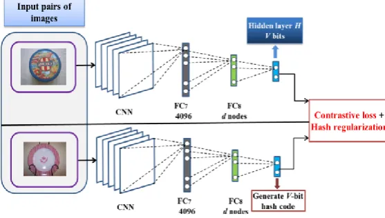
[image:4.612.310.589.612.770.2]Fig. 2 shows the structure of our deep constrained siamese hash coding network. It consists of two symmetrical CNNs which have identical structures and parameters. Pairs of images are input into the network. In the CNNs, we replace the FC8 fully connected layer having 1000 nodes in the AlexNet [37] with the FC8 fully connected layer having d nodes. In contrast with the CNNH which uses hash codes obtained by decomposing the semantic similarity indicator matrix as the supervised signals, we simulate the learning of hash codes by imposing 1 and -1 switching attributes into the last fully connected layer of the CNN. We add a latent layer H with V nodes between the fully connected layer FC8 and the layer of the loss function in the CNN. This latent layer maps the features extracted from the FC7 layer to hash codes. In this latent layer, we use the hyperbolic tangent (tanh) function [41, 42, 43] as the activation function, which is formulated as:
exp( ) exp( ) tanh : ( )
exp( ) exp( )
x x
h x
x x
(1)
where x is an input real value. The range of the tanh function is (-1,1). It is appropriate for the hash coding task.
4
3.2. Loss function
The loss function layer includes the contrastive loss function which measures the similarity of each input pair of images and the regularization function which adds the binary constraint to the output of the latent layer H.
Let {0,1} be the near duplicate indicator, where 1
represents that the two input images are nearly duplicate and 0 represents that they are not nearly duplicate. Let a and b be the V-dimensional vectors output from the latent layers in the two CNNs of our network for a pair of images. These vectors are also called approximate hash codes. The hash codes can be obtained by rounding the components of the approximate hash codes into integers. Let av and bv be the v-th values in a and b. The contrastive loss function is defined as:
2 2
1
1
(1 ) max( , 0)
2
V
c v v v v
v
E a b margin a b
V
(2)where margin is used to adjust the effect of the image pairs which are not nearly duplicate on the entire loss function, i.e., only when the loss is within a specific range (less than margin), the loss is included in the loss function. When the two input images are nearly duplicate, i.e., 1, the contrastive loss is equal to the distance between the approximate hash codes of the two input images, and the contrastive loss is minimized by making the output approximate hash codes as identical as possible. When the two input images are not nearly duplicate, i.e., 0, the contrastive loss is minimized by making the output approximate hash codes as dissimilar as possible. In this way, this contrastive loss function ensures that the learnt hash codes preserve semantic similarity information about the input image pairs.
We define a two-valued constraint term for the loss function, in order to ensure that the approximate hash code components approach 1 or -1 and increase the quality of the produced hash codes. The Hamming distance between the hash codes hi and hj of a pair of images i and j can be represented using the scalar product of hi and hj:
1
dis ( , ) ,
2
H h hi j V h hi j . (3)
The Hamming distance is transformed to be represented using the cosine distance:
dis ( , ) 1 cos( , )
2
H i j i j
V
h h h h (4) where
,
cos( ,i j) i j
i j
h h
h h
h h . (5)
Let ˆa be the vector whose v-th element is av , i.e., ˆ[ ]v av
a . In order to make the hash codes approximate to binary values -1 and 1, we add the following hash regularization term to the loss function:
cos( , )ˆ cos( , )ˆ
h
E a 1 b 1 . (6) where 1 is the V-dimensional vector in which all the entries are 1. We take the cosine distance between the vector whose entries are absolute values of approximate hash codes output from hidden layers H in the network and the vector 1 as a regularization term. As a result, the output
approximate hash codes may approach 1 or -1, and then the quality of the produced hash codes is improved.
We define the entire loss function of our deep constrained siamese hash coding network by EEcEh. This loss function includes near duplication information of image pairs and hash coding constraint. This ensures that near duplicate images have similar hash codes with a high probability.
3.3. Network training
The initial values of the network parameters of the CNNs in our deep constrained siamese hash coding network are taken from the AlexNet which is trained into 1000 classes using the ImageNet dataset. We carry out fine tuning on the AlexNet using the UKbench image dataset and the CIFAR-10 image dataset to obtain the image feature representation for the specific domain of near duplicate image detection.
We transfer the tuned network parameters into our deep constrained siamese hashing network. The near duplicate image dataset is used to train the deep constrained siamese hash coding network. The weights of one of the CNNs in our network are updated using the method in the Caffe [27] CNN deep learning library. The weights of another CNN are just copied from the trained CNN. For a new image, we calculate the output out (Hj) of each node j
in the latent layer H. We binarize out (Hj) into a hash code j
h as follows:
1 ( ) 0
1
j j
out H h
otherwise
. (7)
3.4. Indexing construction
There are two methods to construct a sample index using the learnt network. One method directly uses the hash codes generated from the latent layer H to construct the index structure for the final search. The other method extracts image features from the FC8 layer and then combines the extracted image features with the LSH to construct a LSH-based index structure.
In the first method, given a query image q as well as its learnt hash code hq, according to the distances between
the learnt hash code hq of q and the learnt hash code set
1 2
{ , ,..., }
H N
h h h of the image set, we find the near duplicate candidate image set { ,1 2,..., }
c c c m
I I I for the image q. Then, the final search is carried out on this candidate set. The limitation of the first method is that there is only one hash table for the index structure.
In the second method, features for images are extracted from the FC8 layer of the trained network. Using these extracted features, a LSH-based index is constructed. Given a query image, the near duplicate candidate image set is found based on the constructed index. Let xq and
i
x be the FC8 layer feature vectors of the query image q and the i-th candidate image Iic. The distance between q
and Iic is xqxi . The smaller the distance the more
similar q and Iic are, and the more likely it is that they are
5
As the inputs to our network are pairs of images together with their near duplicate indicators, the features extracted from the network are more appropriate for near duplicate image detection. The binary regularization (6) in the loss function makes the extracted features more effective for constructing LSH.
4. Load-Balanced LSH
As test samples are usually distributed similarly to the training samples, query samples tend to fall into larger buckets in a hash table. This may significantly influence the efficiency of near duplicate image detection. The key idea of load-balanced LSH is to hash the image feature vectors into buckets such that the loads of the buckets balanced. In this way, query samples do not fall into larger buckets and the detection efficiency of the index structure is increased. In the following, we first theoretically derive an upper bound on the hash bucket size, and then use the upper bound to construct a load-balanced LSH.
4.1. Upper bound on hash bucket size
It is necessary to estimate the upper bound LB on the numbers of samples in a bucket for load-balanced LSH. Let
1 2
log(1 / ) log(1 / ) P P
(8)
where P1 and P2 are defined in Section 2. The parameter governs the search performance of the index structure. The smaller the ρ, the more efficient the search.
As stated in [16], given a family of (R, c, P1, P2)-sensitive hash functions, for n d-dimensional samples, the required space for the LSH index structure which is effective for the (R, c)-NN problem is:
1
dnn. (9) From (9), it is seen that the space is determined by ρ. We estimate the an upper bound for ρ according to the lower bound for P1 and the upper bound for P2.
Let τ be the number of degrees of freedom for the chi-squared distribution, and W d be a random projection matrix. For a vector x d , the value
2 2
/
T
W x x is distributed with probability
2 2 2 / T x P x x , where P2( )y for variable y is the
chi-squared distribution: 2 1 2 2 2 ( ) 2 2 y y e P y
. (10)
As proved in [16], the lower bound for P1 is
1 2 1 1 . 2 1 1 1 2 4 P
. (11)
The upper bound for P2 is
2 2 2 2 1 4 P c
.
(12)Substitution of (11) and (12) into (8) yields:
2
2 2
2
1 1
log 2 1
2 4 1 log 1
2 4
1 1 2 log 2 log 1
2 4
. 2 log 2 log 1 4 c c (13)
The right hand term of the equality sign in (13) has the form (e1e2) / (e3e4), where e e e e1, 2, 3, 40. This form is transformed as follows:
2 1
1
1 2 1 2
4
3 4 4 3 1
3 3 3 1 1 1 1 1 e e e
e e e e
e
e e e e e
e e e
. (14)
Taylor series expansion 1/ (1x) 1 O x( ) for variable x yields: 4 4 3 3 1 = 1 1 e O e e e
. (15)
Then, (14) is transformed to
1 2 1 2 4
3 4 3 1 3
= 1 1
e e e e e
O
e e e e e
. (16)
Substitution of the right hand term of the equality sign in (13) into (16) yields:
2
2
1 1 log 1
2 2 log 2 4 1 1 1 log 1 log 1 2 4 4
2 log 2
1 . log 1 4 c O c (17)
The inequality x/ (x 1) log(x 1) x for variable x0 yields: 2 2 2 2 2 2 2 2 2 2 2
1 1 1 1 2
log 1
2 2
4 4 4
log 1
4 4
4
4 4
1 ( 2)( 4 )
4
1 ( 8) 1 1
1 1 .
2 4 c c c c c c c c c O c c (18)
6
2 log 2 log
1 1 1
log 1 log 1
2
4 4
log log
1 4
O
O O
(19)
2 2 2
2 log 2 2 log 2 2 log 2 1
= =
log 1
4 4
O O O O
c c
c
. (20)
Substitution of (18), (19), and (20) into (17) yields
2 2
1 1 log 1 log
1 O 1 O
c c
. (21)
In this way, an upper bound for ρ is obtained [16]. For practical duplicate image detection problems, the number n of images in the database tends to be very large. Therefore, we can consider the upper bound for ρ as n . The degree τ of freedom is directly proportional to n: τn. So,
log
lim 0
n
. (22)
Substitution of (22) into (21) yields
2
1 c
. (23) By substituting (23) into (9), the required storage space for LSH indexing is:
2
1 1/c
dnn . (24) Let B be the maximum number of buckets per hash table. It is usually determined manually according to the number of bits of hash codes and the number of samples. The upper bound on the load-balanced hash bucket size is defined as:
1 1/c2
LB
dn n
LB
. (25)
This means that when n d-dimension samples are stored in L hash tables, each table maintains at most B buckets and each bucket stores at most LB samples. In most cases, it is sufficient to set c=2.
4.2. Load-balanced LSH
The upper bound on the bucket size derived from theoretical analysis is used to construct the load-balanced LSH. It is noted that the buckets are ranked in the ascending order of the hash codes. We design our load-balanced LSH in the following way: If the number of samples placed into the same bucket exceeds the upper bound LB , the extra samples are reassigned into
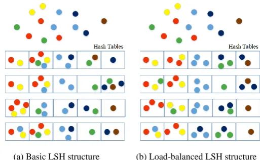
neighboring buckets. In Fig. 3, the load-balanced LSH structure is compared with the basic LSH structure. It is seen that at most three samples are assigned into the same bucket in the load-balanced LSH structure and there are five samples lying in the same bucket in the basic LSH structure.
(a) Basic LSH structure (b) Load-balanced LSH structure Fig. 3. Basic LSH versus load-balanced LSH: Basic LSH may have unbalanced structure which naturally leads to inefficient search. The load-balanced LSH has balanced buckets, which improve the efficiency of the search.
We first initialize the hash mapping functions using the basic LSH family. Then, basic hashing is carried out to map all the samples into buckets without considering the upper bound on the bucket size. When the number of the samples in a bucket exceeds the upper bound, local redistribution is carried out to move some samples in this bucket to neighboring buckets. When all the buckets conform to the size constraint, the load balanced LSH structure is constructed. For detecting near duplicates to a given sample q, the samples in the buckets to which q’s hash codes correspond and the samples in the neighboring buckets are the candidates. To sum up, our load-balanced LSH method consists of the following four steps: initialization of LSH functions, basic hashing, local redistribution of buckets, and neighbor probe search.
4.2.1. Initialization
Our load-balanced LSH uses a family of Hamming LSH functions [10] and a family of Euclidean distance LSH functions [12] to construct the basic LSH mapping function. The Hamming LSH functions map samples into a Hamming space. For a d-dimensional sample x d, the Hamming LSH family is defined as
1
{ : ( )i {0,1}}di
F x , where xi is the i-th component of x and function ( )xi yields a binary code for xi under a given threshold. From F, we randomly select V functions which are concatenated to form a mapping function g() for mapping each sample into a V-bits’ hash code.
A family of the Euclidean distance LSH is a set of functions formulated as:
, ( )
T w b
b r
w x
x (26)
where w is a d-dimension parameter vector with entries generated from the Gaussian distribution, and parameter b is a real number chosen uniformly from the range [0, r] (r is a constant). These hash functions {,b: d Z} map a d-dimensional vector into a set of integers.
4.2.2. Basic hashing
[image:7.612.312.569.43.201.2]7
a bucket g xl( ) in each hash table l, where the upper bound on the bucket size is not considered.
4.2.3. Local redistribution
A local redistribution process is carried out to balance the loads of the buckets. We use the initial hash tables to compute every bucket’s virtual center VC which is the average of the feature vectors of the initial samples in the bucket:
( )
1
t
bucket t t
n
x
VC x (27) where nt is the initial number of samples in bucket t. Then, the buckets in each hash table are checked one by one in the order of hash codes in the hash table. If the number nt of samples in a bucket t exceeds the upper bound LB, we compute the distances between the current samples in the bucket and the virtual center VC of the bucket, and sort the samples by these distances in descending order. Then, the first n t( ) LB samples are chosen and sent to the next bucket t+1. After that, the samples in the next bucket t+1 are processed in the same way as in the bucket t. If the number of the samples in the last bucket exceeds LB, then the chosen farthest samples
are sent to the first bucket, and the local redistribution process restarts from the first bucket. When all buckets conform to the LB constraint, the load balanced LSH construction is finalized. In order to guarantee the stability of the hash buckets and the accuracy of detection, the virtual center VC for each bucket is computed only once for the basic hashing. It is not updated during the local redistribution process. The local redistribution process for each hash table is outlined as follows:
Step 1: Compute the virtual centers of all the buckets based on the results of the basic hashing;
t=1;
Step 2: Compute the distances from the samples in bucket t to the virtual center of the bucket;
Step 3:If n t( ) LB
Choosen t( ) LB samples with farthest distances to the virtual center of bucket t;
If the t-th bucket is the last one
Send these chosen samples to the first bucket; t=1;
Go To Step 2; Otherwise
Send these chosen samples to bucket t+1; t t 1;
Go To Step 2; End If
Otherwise
If the t-th bucket is the last one Go To Step 4
Otherwise
1 t t ;
Go To Step 2; End If
End If Step 4:End
4.2.4. Neighbor-probe search
To cooperate with the local redistribution operation, the load-balanced LSH must probe more than one bucket for approximate nearest neighbors search. Suppose that a query sample q is mapped into the bucket g ql( ) in the l-th hash table. We probe the bucket g pl( ) and the next buckets to find the near duplicate samples. The number of the buckets next to the bucket h ql( ) is determined by:
LB
LB Ml
(28)
where Ml is the mean of the numbers of samples in the buckets in the l-th hash table. The more the mean number of samples in buckets, the more the buckets to be searched. In this way, the near duplicate images can be detected efficiently.
4.2.5. Discussion
The CNN model can be trained incrementally by using the previous models to initialize the new model. Our indexing construction method currently cannot be incremental. However, the construction process is very efficient. The indexing structure can be reconstructed very efficiently. We will study how to incrementally construct the indexing structure in our future work.
5. Experiments
We adopted the following three public benchmark image datasets to evaluate the effectiveness of our deep constrained siamese hash coding network and load-balanced LSH:
The CIFAR-10 dataset: It consists of 60,000 color images with size 32×32. These images have 10 classes, and each class contains 6,000 images. The dataset was divided into a training set with 50,000 images and a test set with 10,000 images. The images from the same class are treated as near duplicated. Since the experiments were conducted to evaluate the effectiveness of different hashing methods, the experimental findings are also referable to other treatments of near duplication.
The UKbench dataset [17]: It consists of 10,200 color images with size 640×480. It contains 2,550 different scenes. Each scene has four near duplicate images. The dataset was divided into a training set with 7,550 images and a test set with 2,550 images.
8
In these datasets, there are many similar images which produce a number of very large buckets using the basic hashing, making the load of the buckets unbalanced.
On the CIFAR-10 dataset, the mean Relevance Precision (mRP) was used as the metric for accuracy evaluation. Let k be the number of image candidates returned by the index structure. The mRP is defined as:
1
1
RP ( )
k
i
m Rel i k
(29)where Rel i( ) is 1 if the i-th returned candiate is a duplicate of the query image, otherwise it is 0. This is an absolute measure of accuracy.
On the UKbench dataset, the relative mRP, the absolute precision N-S (Normalized Similarity) score, and the acceleration factor were used as metrics for performance evaluation. Let indexing be the number of the correct candidates in the top k candidates returned by the indexing method. Let exhaustive be the number of the correct candidates in the top k candidates returned by exhaustive search. The relative mRP is defined as:
RP( ) indexing
exhaustive
m relative
. (30)
This mRP depends on the accuracy of exhaustive search, i.e., the results of exhaustive search are used as the baseline. Let 4
i
be the number of the correct results for image i in the top 4 returned candidates. The N-S score is defined as:
4 1
1 N-S score
4
T
n i i T
n
(31)where nT is the number of the images in the test set. The N-S score is an absolute precision. The acceleration factor is defined as n n/ r, where n is the total number of images in the dataset and nr is the number of image candidates returned by the index structure. Exhausive search examines all the n samples, so the acceleration factor is the detection efficiency estimation relative to exhaustive search.
5.1. Deep constrained siamese hash coding
network
Two indexing methods have been constructed. One method (the first method) directly uses the hash codes output from the deep constrained siamese hash coding network to construct the indexing structure. Another method (the second method) uses the features extracted from the FC8 layer in the network to construct a LSH-based index structure. The value of d for the FC8 layer is set to 1000.The two methods were compared with the following indexing methods:
Traditional feature-based index structures, namely ITQ in [29], KSH in [30]: Each image was represented by a 32-dimensional gist feature vector [19]. These features were used to construct the index structure.
Deep feature and LSH combined index structure: We used the training samples in the CIFAR-10 dataset to tune the AlexNet. Image features were extracted from the FC7 layer in the tuned network. Then, LSH was used to index the images.
Convolutional neural network hashing (CNNH)-based indexing structure: The near
[image:9.612.325.563.112.224.2]duplicate indicator matrix-based deep hash coding learning network [25] was used to generate 48-bit hash codes for images.
Table 1. Comparison between different features-based indexing structures with different bit lengths on the CIFAR-10 dataset
Methods mRP
12-bit 24-bit 32-bit 48-bit The first method 0.76 0.77 0.787 0.79 The second method 0.876 0.88 0.88 0.898
AlexNet +
load-balanced LSH 0.62 0.64 0.645 0.65 CNNH 0.539 0.576 0.572 0.589
KSH 0.303 0.337 0.346 0.356 ITQ 0.162 0.169 0.172 0.175
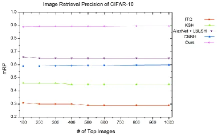
On the CIFAR-10 dataset, 5000 images were randomly selected from each class, 50000 images in total, as the training images. For training the network, each image pair’s label indicating whether the two images are duplicated was determined by the ground truth of the images. We selected 1000 images randomly from each of the 10 classes, 10000 images in total, as the set of query images. Table 1 shows the results of different indexing methods with different bit lengths for the hash codes. It shows how our methods compare with ITQ, KSH, CNNH, and the tuned AlexNet and LSH combined method. Fig. 4 shows the mRPs of the different methods for 48-bit hash codes when the number of returned images changes. It is seen that our methods yield more accurate results than the competing methods. The results of the network and LSH combined method (the second method) are more accurate than the results of our method only based on the hash codes output from our network (the first method). This is because the non-LSH method only produces one hash table while the network and LSH combined method produces a number of hash tables. The reason why the CNNH-based method does not yield results comparable to the results of our methods is the information loss in the decomposition of the near duplication indicator matrix into hash codes.
Fig. 4. The results for the 48-bit hash codes on the CIFAR dataset.
[image:9.612.334.553.529.664.2]9
[image:10.612.352.535.50.187.2]method, where the number L of hash tables is 20. Fig. 6 shows the curves of the relative mRPs versus the acceleration factors for the AlexNet features and LSH combined methods and our network and LSH combined methods. The relative mRP achieves 1.0 means that the hashing process does not reduce the mRP value compared with the exhaustive searching. It is seen that the features extracted from our neural network yield more accurate results than the traditional SIFT BoFs and the features extracted from traditional deep neural network, i.e., under the same acceleration factor the features extracted from our neural network obtain higher mRPs. This illustrates that our deep constrained siamese hash coding network effectively learns the features which are appropriate for constructing LSH index structures.
Fig. 5. Comparison between the features from the FC8 layer in our network and the SIFT-based BoFs on the UKbench dataset.
Fig. 6. Comparison between the features extracted from our hash coding network and the features from the tuned AlexNet on the UKbench dataset.
5.2. Load-balanced LSH
We first verify the effectiveness of the upper bound on the load-balanced bucket size, then the effectiveness of the load-balanced LSH.
5.2.1. Analysis of load-balanced upper bound
[image:10.612.54.286.236.366.2]The key idea of our load-balanced LSH is to hash the image feature vectors into buckets which contain an appropriate number of samples. It is important to verify the effectiveness of the theoretically derived value of the parameter LB in designing the load balanced LSH. We explored the effect of LB on the accuracy and efficiency for searching near duplicate images on the UKbench dataset.
Fig. 7. The results of the load-balanced Euclidean LSH with different values of LB (L=20).
We extracted 320-dimensional gist features [19] for each image. We mapped all the 10,200 images in the dataset into each of 20 hash tables. Each table contains at most 2000 buckets. Based on (25) in Section 4.1, the threshold
LB is estimated as:
1+0.25
320 10200+10200
84
2 0 0
=
0 2 0
LB
. (32)
The Euclidean distance-based LSH was used. Fig. 7 shows the curves of the relative mRP versus the acceleration factor for searching near duplicate images when LB takes the
values 50, 60, 84, 100, 120, and
. When LB is infinite,i.e., there is no limit to the load in a bucket, the load-balanced LSH is reduced to the basic LSH. From the results, we observe that when LB is 84 the best detection accuracy and efficiency are achieved. This clearly illustrates the effectiveness of the theoretically derived value of the upper bound LB.
5.2.2. Performance comparison with basic LSH
In order to show the effectiveness of our proposed load-balanced LSH for near duplicate image detection, we compared our load-balanced LSH with the basic LSH on the three benchmark dataset: the CIFAR dataset, the UKbench dataset, and the INRIA Copydays dataset.
1) The CIFAR dataset
Fig. 8. Comparison between our load-balanced Hamming LSH and the Hamming LSH when deep features are used (L=20).
[image:10.612.51.287.402.535.2] [image:10.612.344.521.558.695.2]10
network. The results are shown in Fig. 8. It is seen that when the features from AlexNet or the features from our neural network are used, under the same acceleration factor the load-balanced Hamming LSH yields more accurate results than the Hamming LSH, and under the same mRP the load-balanced Hamming LSH works more rapidly.
2) The UKbench dataset
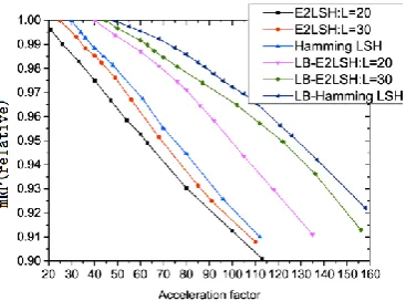
On the UKbench dataset, we compared our load-balanced LSH with the basic LSH using two global features: the 320-dimensional gist features [19] and the 400-dimensional SIFT [20]-based BoFs. The Hamming LSH (HLSH) and the Euclidean LSH (E2LSH) were used. For the Euclidean LSH, the number of hash tables was varied for different types of features to obtain a range of performances. For the gist features, the number of hash tables was set to 20 and 30, and correspondingly the upper bound LB on the hash bucket was 84 and 54. For the
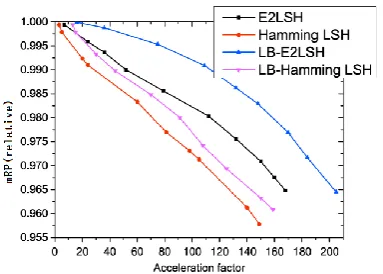
[image:11.612.331.554.74.194.2]SIFT-based BoFs, the number of hash tables was set to 15 and 20, and correspondingly the upper bound on the bucket size was 134 and 100. Figs. 9 and 10 show the results in terms of relative mRP versus acceleration factor for the gist features and the SIFT-based BoFs, respectively. From the comparisons, we observe that, at the same detection accuracy, the load-balanced Euclidean/Hamming LSH has a higher acceleration factor than the basic Euclidean/Hamming LSH. These results clearly illustrate the effectiveness of the load balanced LSH.
[image:11.612.330.552.277.424.2]Fig. 9. Comparisons between our load-balanced LSH and basic LSH for the gist features on the UKbench dataset.
Fig. 10. Comparisons between our load-balanced LSH and the basic LSH for the SIFT BoFs on the UKbench dataset.
On the UKbench dataset, we compared our load-balanced LSH with the basic LSH for the tuned AlexNet features and the features extracted from our deep constrained siamese hash coding network. The results are
shown in Fig. 11. It is seen that with the same features our load-balanced LSH outperforms the classic LSH.
Fig. 11. Comparisons between our load-balanced LSH and the basic LSH for the deep learning features on the UKbench dataset.
Table 2. Comparison between the Euclidean LSH and our load-balanced Euclidean LSH based on the features obtained by early fusion of color, LBP and RootSIFT on the UKbench dataset
Evaluation criteria N-S score Image cand. Acce.factor
Basic E2LSH
V=24 3.462 939.0 10.9
V=25 3.507 953.0 10.7
V=26 3.493 943.0 10.8
V=27 3.484 931.5 11.0
V=28 3.442 883.5 11.5
Proposed LB-E2LSH
V=24 3.490 620.8 16.4
V=25 3.508 636.2 16.0
V=26 3.506 634.8 16.1
V=27 3.495 625.6 16.3
V=28 3.494 621.7 16.4
Table 3. Comparison between the Hamming LSH and our load-balanced Hamming LSH based on the features extracted from our deep constrained siamese hash coding network on the UKbench dataset
Evaluation criteria N-S score Image cand. Acce.factor Basic
HLSH
V=12 3.24 638.0 16
V=24 3.45 653.0 15.6
V=32 3.61 643.0 15.9
V=48 3.61 639.5 15.9 Proposed
LB-HLSH
V=12 3.47 421 24.2
V=24 3.58 436.6 23.4
V=32 3.66 434.8 23.5
V=48 3.65 429 23.7
[image:11.612.79.263.392.528.2] [image:11.612.333.553.484.602.2] [image:11.612.79.257.562.693.2]11
designed to detect near duplicate images efficiently, the N-S scores of our load balanced Euclidean LSH exceed the score of 3.17 for the min-hash in [6] and 3.42 for the BoF in [24] on the UKbench dataset. We also combined the features extracted from our deep constrained siamese hash coding network with the Hamming LSH (HLSH) and the load-balanced Hamming LSH (LB-HLSH) to detect near duplicate images. The results are shown in Table 3. It is also seen that the load-balanced Hamming LSH is more efficient and more accurate.
3) The INRIA Copydays dataset
On the INRIA Copydays dataset, we made the comparison based on the 320-dimensional gist features and the 400-dimensional SIFT-based BoFs. The Hamming LSH and the Euclidean LSH were used to compare the load balanced LSH with the basic LSH. For the gist features, the number of hash tables was set to 20, giving a value of 27 for LB. For the SIFT-based BoFs, the number of hash
tables was set to 30, with LB equal to 34. Figs. 12 and 13
[image:12.612.73.265.341.478.2]show the results for the gist features and the SIFT-based BoFs respectively. These results show the good performance of the load balanced LSH.
[image:12.612.79.246.525.647.2]Fig. 12. Comparisons between our load-balanced LSH and the basic LSH for the gist features on the INRIA Copydays dataset.
Fig. 13. Comparisons between our load-balanced LSH and the basic LSH for the SIFT-based BoFs on the INRIA Copydays dataset.
5.3. Remark
In the experiments, different datasets with different numbers of samples were used, and different dimensions of feature vectors were used. In all the results, the load-balanced LSH is more efficient than the basic LSH. This clearly shows the effectiveness of the upper bound of the load-balanced hash bucket size.
6. Conclusion
We have proposed a deep constrained siamese hash coding network to which binary constrained regularization is added. The training of the network is simple and the network is able to learn effective image features which are appropriate for detecting near duplicate images and for constructing LSH-based indexing. We have further proposed a load-balanced LSH method for the efficient and effective detection of near duplicate images. Our load balanced LSH guarantees to map images into buckets in a balanced way and to probe an appropriate number of neighboring buckets for detection. This accelerates the detection and also obtains good accuracy. Therefore, our load-balanced LSH is efficient and flexible in contrast with the basic LSH. The experimental results on three benchmark datasets demonstrate the effectiveness of our deep constrained siamese hash coding network and efficiency of our load-based LSH.
References
1. A. Joly, O. Buisson, and C. Frelicot, “Content-based copy retrieval using distortion-based probabilistic similarity search,”
IEEE Trans. on Multimedia, vol. 9, no. 2, pp. 293-306, 2007. 2. Z. Wu, Q. Xu, S. Jiang, Q. Huang, P. Cui, and L. Li, “Adding
affine invariant geometric constraint for partial-duplicate image retrieval,” in Proc. of International Conference on Pattern Recognition, pp. 842-845, Aug. 2010.
3. Y. Lin, C. Xu, L. Yang, Z. Lin, and H. Zha, “L1-norm global geometric consistency for partial-duplicate image retrieval,” in Proc. of IEEE International Conference on Image Processing, pp. 3033-3037, Oct. 2014.
4. Y. Ke, R. Sukthankar, and L. Huston, “Efficient near-duplicate detection and sub-image retrieval,” in Proc. of ACM International Conference on Multimedia, pp. 869-876, Jan. 2004. 5. W. Zhao, C. Ngo, H. Tan, and X. Wu, “Near-duplicate keyframe identification with interest point matching and pattern learning,”
IEEE Trans. on Multimedia, vol. 9, no. 5, pp. 1037-1048, 2004. 6. O. Chum, J. Philbin, and A. Zisserman, “Near duplicate image
detection: min-hash and tf-idf weighting,” in Proc. of British Machine Vision Conference, pp. 50.1-50.10, 2008.
7. Z. Xu, H. Ling, F. Zou, Z. Lu, and P. Li, “Robust image copy detection using multi-resolution histogram,” in Proc. of ACM International Conference on Multimedia Information Retrieval, pp. 129-136, 2010.
8. Y. Lei, G. Qiu, L. Zheng, and J. Huang, “Fast near-duplicate image detection using uniform randomized trees,” ACM Trans. on Multimedia Computing, Communications, and Applications, vol. 10, no. 4, Article no. 35, 2014.
9. M. Wang W. Zhou, Q. Tian, and H. Li, “A General framework for linear distance preserving hashing,” IEEE Trans. on Image Processing, Accepted, 2017.
10.A. Gionis, P. Indyk, and R. Motwani, “Similarity search in high dimensions via hashing,” in Proc. of International Conference on Very Large Data Bases, pp. 518-529, 1999.
11.P. Indyk and R. Motwani, “Approximate nearest neighbors: towards removing the curse of dimensionality,” in Proc. of ACM Symposium on Theory of computing, pp. 604-613, 1998.
12.M. Datar, N. Immorlica, P. Indyk, and V.S. Mirrokni, “Locality-sensitive hashing scheme based on p-stable distributions,” in Proc. of ACM Symposium on Computational Geometry, pp. 253-262, 2004.
13.B. Kulis and K. Grauman, “Kernelized locality-sensitive hashing for scalable image search,” in Proc. of IEEE International Conference on Computer Vision, pp. 2130-2137, 2009.
12 sensitive hashing for duplicate image retrieval,” in Proc. of IEEE International Conference on Image Processing, pp. 2461-2464. Sep. 2011.
15.Q. Lv, W. Josephson, Z. Wang, M. Charikar, and K. Li, “Multi-probe LSH: efficient indexing for high-dimensional similarity search,” in Proc. of International Conference on Very Large Data Bases, pp. 950-961, 2007.
16.A. Andoni and P. Indyk, “Near-optimal hashing algorithms for approximate nearest neighbor in high dimensions,”
Communications of the ACM, vol. 51, no. 1, pp. 117-122, Jan. 2008.
17.D. Nister and H. Stewenius, “Scalable recognition with a vocabulary tree,” in Proc. of IEEE Conference on Computer Vision and Pattern Recognition, pp. 459-468, Oct. 2006.
18.M. Douze, H. Jegou, H. Sandhawalia, L. Amsaleg, and C. Schmid, “Evaluation of GIST descriptors for web-scale image search,” in Proc. of ACM International Conference on Image and Video Retrieval, Article no. 19, 2009.
19.A. Oliva and A.B. Torralba, “Modeling the shape of the scene: a holistic representation of the spatial envelope,” International Journal of Computer Vision, vol. 42, no. 3, pp. 145-175, 2001. 20.D.G. Lowe, “Distinctive image features from scale-invariant
keypoints,” International Journal of Computer Vision, vol. 60, no. 2, pp. 91-110, 2004.
21.T. Ojala, M. Pietikainen, and T. Maenpaa, “A generalized local binary pattern operator for multiresolution gray scale and rotation invariant texture classification,” in Proc. of IEEE International Conference on Advances in Pattern Recognition, pp. 399-408, May 2001.
22.R. Arandjelovic and A. Zisserman, “Three things everyone should know to improve object retrieval,” in Proc. of IEEE Conference on Computer Vision and Pattern Recognition, pp. 2911-2918, June 2012.
23.H. Jegou, F. Perronnin, M. Douze, J. Sanchez, P. Perez, and C. Schmid, “Aggregating local image descriptors into compact codes,” IEEE Trans. on Pattern Analysis and Machine Intelligence, vol. 34, no. 9, pp. 1704-1716, 2012.
24.H. Jegou, M. Douze, and C. Schmid, “Improving bag-of-feature for large scale image search,” International Journal of Computer Vision, vol. 87, no. 3, pp. 316-336, 2010.
25.R. Xia, Y. Pan, H. Lai, C. Liu, and S. Yan, “Supervised hashing for image retrieval via image representation learning,” in Proc. of AAAI Conference on Artificial Intelligence, pp. 2156-2162, 2014. 26.W.-J. Li, S. Wang, and W.-C. Kang, “Feature learning based deep supervised hashing with pairwise labels,” in Proc. of International Joint Conference on Artificial Intelligence, pp. 1711-1717, 2016.
27.Y. Jia, E. Shelhamer, J. Donahue, S. Karayev, J. Long, R. Girshick, S. Guadarrama, and T. Darrell, “Caffe: Convolutional architecture for fast feature embedding,” in Proc. of ACM international conference on Multimedia, pp. 675-678, 2014. 28.S. Korman and S. Avidan, “Coherency sensitive hashing,” IEEE
Trans. on Pattern Analysis and Machine Intelligence, vol. 38, no. 6, pp. 1099-1112, June 2016.
29.Y. Gong, S. Lazebnik, A. Gordo, and F. Perronnin, “Iterative quantization: a procrustean approach to learning binary codes for large-scale image retrieval,” IEEE Trans. on Pattern Analysis and Machine Intelligence, vol. 35, no. 12, pp. 2916-2929, Dec. 2013.
30.W. Liu, J. Wang, R. Ji, Y.-G. Jiang, and S.-F. Chang, “Supervised hashing with kernels,” in Proc. of IEEE Conference on Computer Vision and Pattern Recognition, pp. 2074-2081, 2012.
31.C. Kim, “Content-based image copy detection,” Signal Process: Image Communication, vol. 18, no. 3, pp. 169-181, 2003. 32.M.-N. Wu, C.-C. Lin, and C.-C. Chang, “Content-based image
copy detection,” Journal of Systems and Software, vol. 80, no. 7, pp. 1057-1069, 2007.
33.K. Li, G.-J. Qi, J. Ye, and K.A. Hua, “Linear subspace ranking
hashing for cross-modal retrieval,” IEEE Trans. on Pattern Analysis and Machine Intelligence, vol. 39, no. 9, pp. 1825-1838, Sep. 2017.
34.J. Sivic and A. Zisserman, “Video Google: a text retrieval approach to object matching in videos,” in Proc. of IEEE International Conference on Computer Vision, pp. 1470-1477, 2003.
35.Y. Lei, Y. Wang, and J. Huang, “Robust image hash in radon transform domain for authentication,” Signal Process: Image Communication, vol. 26, no. 6, pp. 280-288, 2011.
36.L. Zheng, Y. Lei, G. Qiu, and J. Huang, “Near-duplicate image detection in a visually salient Riemannian space,” IEEE Trans. on Information Forensics and Security, vol. 7, no. 5, pp. 1578õ1593, 2012.
37.A. Krizhevsky, I. Sutskever, and G.E. Hinton, “ImageNet classification with deep convolutional neural networks,” in Proc. of Advances in Neural Information Processing Systems, pp. 1097-1105, 2012.
38.M. Oquab, L. Bottou, I. Laptev, and J. Sivic, “Learning and transferring midlevel image representations using convolutional neural networks,” in Proc. of IEEE Conference on Computer Vision and Pattern Recognition,pp. 1717-1724, 2014.
39.M.D. Zeiler and R. Fergus, “Visualizing and understanding convolutional networks,” in Proc. of European Conference on Computer Vision, pp. 818-833, 2014.
40.O. Russakovsky, J. Deng, H. Su, J. Krause, S. Satheesh, S. Ma, Z. Huang, A. Karpathy, A. Khosla, M. Bernstein, A.C. Berg, and L. Fei-Fei, “ImageNet large scale visual recognition challenge,”
International Journal of Computer Vision, vol. 115, no. 3, pp. 211-252, Dec. 2015.
41.Z. Chen, J. Lu, J. Feng, and J. Zhou, “Nonlinear discrete hashing,”
IEEE Trans. on Multimedia, vol. 19, no. 1, pp. 123-135, Jan. 2017.
42.V.E. Liong, J. Lu, G. Wang, P. Moulin, and J. Zhou, “Deep hashing for compact binary codes learning,” in Proc. of IEEE Conference on Computer Vision and Pattern Recognition, pp. 2475-2483, 2015.
43.Z. Chen and J. Zhou, “Collaborative multiview hashing,” Pattern Recognition, vol. 75, pp. 149-160, Mar. 2018.
44.G. Lin, C. Shen, D. Suter, and A.V.D. Hengel, “A general two-step approach to learning-based hashing,” in Proc. of IEEE International Conference on Computer Vision, pp. 2552-2559, 2013.
45.X. Li, G. Lin, C. Shen, A. Hengel, and A. Dick, “Learning hash functions using column generation,” in Proc. of International Conference on Machine Learning, pp. 142-150, 2013.
Weiming Hu received the Ph.D. degree from the department of computer science and engineering, Zhejiang University in 1998. From April 1998 to March 2000, he was a postdoctoral research fellow with the Institute of Computer Science and Technology, Peking University. Now he is a professor in the Institute of Automation, Chinese Academy of Sciences. His research interests are in visual motion analysis and recognition of web objectionable information.
13 problems related to classification and hashing.
Junliang Xing received the B.S. degree in computer science and mathematics from Xi'an Jiaotong University, Shaanxi, China, in 2007, and the Ph.D. degree in computer science from Tsinghua University, Beijing, China, in 2012. He is currently an assistant professor with the National Laboratory of Pattern Recognition, Institute of Automation, Chinese Academy of Sciences, Beijing, China. His current research interests mainly focus on computer vision problems related to faces and humans.
Liang Sun received the B.S. degree in Automation from Hefei University of Technology, Hefei,China, in 2016. He is a Joint training of graduate students with University of Science and Technology of China, Hefei, China and the National Laboratory of Pattern Recognition, Institute of Automation, Chinese Academy of Sciences, Beijing, China. His current research interests mainly focus on deep learning and video captioning.
Zhaoquan Cai received the bachelor degree in Computer Science and Technology from South China University of Technology in 1998, and the master degree in Computer Science and Technology from Huazhong University of Science and Technology, Wuhan, China in 2006. He is currently the director of the Science Research Management Department in Huizhou University. His current research interests mainly focus on computer networks, intelligent computing and database.