BIROn - Birkbeck Institutional Research Online
Cieslak, A. and Povala, Pavol (2013) Information in the term structure of
yield curve volatility. Working Paper. Birkbeck College, University of London,
London, UK.
Downloaded from:
Usage Guidelines:
Please refer to usage guidelines at or alternatively
Information in the term structure of
yield curve volatility
Anna Cieslak
and
Pavol Povala
∗We study information in the volatility of US Treasuries. We propose a no-arbitrage term structure model with a stochastic covariance of risks in the economy, and estimate it using high-frequency data and options. We identify volatilities of the expected short rate and of the term premium. Volatility of short rate expectations rises ahead of recessions and during stress in financial markets, while term premium volatility increases in the aftermath. Volatile short rate expectations predict economic activity independently of the term spread at horizons up to one year, and are related to measures of monetary policy uncertainty. The term premium volatility comoves with a more general level of economic policy uncertainty. We also study channels through which volatility affects model-based inference about the yield curve.
This version: September, 2013 JEL classification: E43, C51
∗Cieslak is at the Northwestern University, Kellogg School of Management. Povala is at the University of London, Birkbeck.
A vast literature studies and decomposes the information contained in the nominal Treasury yield curve. Perspectives vary from latent factors, reduced-form macro-finance models, through structural settings but most of the time they serve the objective of understanding the Treasury risk premia and short rate expectations. The majority of the recent term structure literature has tackled this and related questions assuming constant volatility. That focus can be justified with tractability and the known difficulties with the joint modeling of the first and second moments of yields. Consequently, relatively little is known about information embedded in the Treasury market volatility.
As the largest and the most liquid debt market in the world, US Treasuries provide investors, central banks and governments worldwide not only with the store of value and liquidity but also serve as the main source of collateral in various transactions. The fluctuations in Treasury yields and in their volatility have impact on a range of asset markets. A rise in interest rate volatility may signal macroeconomic uncertainty, but might also lead to an increase in haircuts for Treasury bonds used as collateral in about half of the repo transactions, and thus diminish the lending capacity in the financial system.1 These considerations make the understanding of interest rate volatility especially compelling.
In this paper, we ask what we can learn about the term structure and the economy by studying the time-varying second moments of the Treasury yield curve. Relative to the previous literature, our approach is comprised of several new elements: First, to identify the properties of interest rate volatility, we rely on nearly 20 years worth of high-frequency data on transactions in the US Treasury market. The dataset allows us to construct the realized covariance matrix of zero-coupon yields across different maturities. Additionally, we augment the realized co-volatility estimates with information from Treasury derivatives, covering risk-adjusted market expectations of volatility at several points along the yield curve. Second, we propose a no-arbitrage term structure model that is able to accommodate the multivariate dynamics of yield volatilities that we find in the data. In particular, we model the entire stochastic covariance matrix of risks in the economy. This setting imposes a structure on our data through a joint estimation that involves yields, their realized
1According to SIFMA quarterly report, in the third quarter of 2010 the outstanding volume of repos and
covariance matrix and implied volatilities. With its guidance, we uncover and interpret a factor structure in interest rate volatility.
Our first set of results focuses on the economic interpretation of the volatility dynamics. Interest rate volatility moves around because of either volatile short rate expectations or volatile risk premia. To the extent that short rate expectations reflect market expectations about the path of monetary policy, understanding fluctuations of interest rate volatility over the business cycle is informative about the amount of uncertainty surrounding that path.
The model decomposes information in realized covariances and implied volatilities into three components: two volatility states, which we term as the short- and long-end volatility, and a covariance state. The short-end volatility is the key element driving the variance of short rate expectations; the long-end volatility instead determines the variance of the term premia. The covariance state generates the conditional comovement between shocks to short rate expectations and premia. We study the empirical properties of these factors at different maturities and over time. Perhaps not surprisingly, the volatility of the two-year bond is mostly determined by the expectations part, while that of the ten-year bond by the term premium part. Volatile short rate expectation rather than term premia produce the well-known hump in the unconditional term structure of yield volatilities at maturity of about three years. In terms of time series properties, we find that the short rate expectations component of volatility is shorter lived and less persistent, with a half-life of about half that of the term premium volatility.
By modeling the stochastic covariance of risks in the yield curve, we are able to study the comovement between short rate expectations and the term premia. In this way, we cast new light on the tradeoffs faced by the Fed. During the last two decades, the model implies that the conditional correlation between the term premium and short rate expectations is on average slightly positive (average correlation is below 0.2) but highly time varying. Interestingly, the correlation increases during the long easing episode in 2000/03, and declines afterwards. The model interprets the Greenspan’s conundrum period as a gradual decline of the correlation between short rate expectations and the term premium.
As part of our analysis, we document how volatility dynamics determined by the model can be linked to macro-finance observables. We verify our interpretation of volatility states using common uncertainty measures that are independent of asset prices. Specifically, we find that the short-end (short rate expectations) volatility comoves with the level of uncertainty about the monetary policy visible in professional survey forecasts, whereas the long-end (term premium) volatility is correlated with the amount of the economic policy uncertainty. The latter is measured with the index of Baker, Bloom, and Davis (2013), and captures mostly the uncertainty about taxes, spending and regulatory policies.
Our results suggest that interest rate volatility contains additional information about the economy that cannot be read from the standard yield curve factors alone. It is known that the slope of the term structure predicts economic activity at horizons between one and two years ahead. We show that, over our sample period, the short-end volatility forecasts growth at horizons up to one year, and its forecasting power is separate from that of the slope. This is in line with short-rate expectations becoming increasingly volatile ahead of bad times.
We also establish how interest rate volatility interacts with liquidity in asset markets. There exists an interesting lead-lag relationship between yield curve volatility and market-wide liquidity proxies as constructed by Pastor and Stambaugh (2003) for the equities, and Hu, Pan, and Wang (2012) for Treasury bonds. We find that deteriorating liquidity conditions forecast an increase in the term premium (long-end) volatility with a lag up to above a year. However, we fail to find a similarly strong link with the volatility of short rate expectations. Rather, similar to its ability to predict slowdown in economic activity, an increased short-end volatility preempts worsening liquidity several quarters ahead.
effect on the cross sections of yields. In that we do not impose any a priori restrictions and, at the same time, ask the model to match the volatility in the data, this result extends the evidence in the literature on unspanned or hidden factors. For instance, consistent with the notion of hidden factors, we find that the short-end volatility has less than one basis point cross-sectional effect on the term structure, but it contains predictive information about the future macro environment. Second, while we allow volatility risk to be priced, and to impact bond risk premia, we find also this channel not to be quantitatively important. The Treasury term premium can be associated almost entirely with the priced yield curve shocks rather than volatility shocks. Likewise, we do not find evidence that volatility generates predictable variation in bond excess returns in the last two decades. Nevertheless, the model generates realistic dynamics of bond variance risk premium implying that on average investors pay a premium to hedge interest rate volatility risk. The variance risk premium is the highest at the three-year maturity and declines afterwards.
Related literature
Our paper is related to the literature on realized volatility, term structure models with stochastic volatility, and the research into the role of US Treasury bonds in liquidity provision.
Recent advances in high-frequency econometrics have encouraged a model-free look into the statistical properties of bond volatility. Andersen and Benzoni (2010) test empirically the volatility implications of affine term structure models (ATSMs) using realized volatility over the 1991–2000 period. In line with the early evidence in Collin-Dufresne and Goldstein (2002), they find that systematic volatility factors are largely independent from the cross section of yields, and call for extensions of the popular models in the volatility dimension.2
In the latent factor domain, several recent papers document that benchmark models with stochastic volatility face difficulties in explaining variation in yield volatility, and those difficulties become increasingly severe at the long end of the yield curve. Collin-Dufresne, Goldstein, and Jones (2009, CDGJ) report that over the 1988–2005 sample, the variance series generated by a standard three-factor model, A1(3), are essentially unrelated to the model-free conditional volatility measures. Using the same model, Jacobs and Karoui (2009) find a correlation between model-implied and EGARCH volatility reaching up to
2
75% over the 1970–2003 period. However, in the more recent sample (1991–2003) this correlation breaks down and becomes negative at the long end of the curve. In a study of Japanese yields at the zero lower bound, Kim and Singleton (2012) arrive at a similar conclusion based on several models. These authors suggest that additional volatility factors may be needed to explain the volatility at the long maturity range. We contribute to this discussion by proposing a new term structure model that accommodates the multivariate nature of yield volatilities, and support its estimation with the information from the realized covariance matrix of yields and implied volatilities. We find that these two elements of our approach alleviate the problems with generating realistic volatility dynamics documented in the literature, allowing us to focus on their economic interpretation.
Andersen, Bollerslev, Diebold, and Vega (2007) and Jones, Lamont, and Lumsdaine (1998) show that relative to other liquid asset markets, bond prices tend to provide a clear and pronounced reaction to economic news. These studies suggest that a rich economic content is present in bond volatilities. The model-based decomposition of the yield volatility allows us to study how its distinct components related to short rate expectations and term premia interact with measures of economic and financial conditions.
Several studies introduce stochastic volatility into macro-finance term structure models.3 Adrian and Wu (2009) and Campbell, Sunderam, and Viceira (2013) highlight the impor-tance of a stochastic covariance between the real pricing kernel and expected inflation in determining excess bond returns. These models attach economic labels to different yield volatility components. However, understanding the dynamics and the determinants of the yield volatility per se is not in their direct focus. Our paper is the first to study the properties of volatilities decomposing them into risk premium and short rate expectations components. We show that such a decomposition yields new insights about risks in Treasury bonds that cannot be in inferred from yield levels alone.
Given the role that US Treasuries play in the financial system, it is important to understand how volatility of bonds relates to the fluctuations in demand for liquidity and collateral. A growing literature focuses on extracting information about liquidity from the cross section of bonds with different age (e.g. Vayanos and Weil, 2008; Fontaine and Garcia, 2012). Recently, Hu, Pan, and Wang (2012) compose a noise illiquidity measure as an average yield pricing error of Treasury bonds. Using our model-based decomposition of yield volatility,
3
we observe differences in the way volatility components comove with liquidity conditions at leads and lags. Since each volatility state that we identify has an economically different interpretation, these results suggest that complex interactions between liquidity and interest rate volatility may be at work.
I. Data
I.A. High-frequency bond data and zero-coupon yield curve tick-by-tick
We use high-frequency nominal US Treasury bond data spanning two long expansions, two recessions and three monetary policy cycles. We obtain 19 years’ worth of high-frequency price data of Treasury securities from January 1992 through December 2010 by splicing historical observations from two inter-dealer broker platforms: GovPX (1992:01–2000:12)4 and BrokerTec (2001:01–2010:12). The merged data set covers about 60% of transactions in the secondary US Treasury bond market. In total, we work with around 50 million on-the-run Treasury bond quotes/transactions (Mizrach and Neely, 2006; Fleming and Mizrach, 2009).
GovPX comprises Treasury bills and bonds with maturities three, six and 12 months, and two, three, five, seven, ten and 30 years. BrokerTec, instead, contains only Treasury bonds with maturities two, three, five, seven (in part of the sample), ten and 30 years. In the GovPX period, we identify on-the-run securities and use their mid-quotes for further analysis. Unlike GovPX, which is a voice-assisted brokerage system, BrokerTec is a fully electronic trading platform attracting vast liquidity and thus allowing us to consider traded prices of on-the-run securities. Roughly 95% of trading occurs between 7:30AM and 5:00PM EST (e.g. Fleming, 1997), which we treat as the trading day. We sample bond prices at ten-minute intervals taking the last available price for each sampling point. More information on our dataset is provided in Appendix I.A
The raw data set contains coupon bonds. We use equally-spaced high-frequency price data to obtain the zero coupon yield curve for every sampling point following the procedure of Fisher, Nychka, and Zervos (1994). In order to anchor the short end of the maturities range in the construction of the zero-coupon curve in the BrokerTec period, we supplement the high-frequency data with the daily observations of the three-month T-bill rate available from the Fed’s H.15 statistical release. Even though our zero-coupon yield curve spans
4
maturities below two years, in the estimation of realized volatilities we use the two-year yield as the shortest maturity due to the lack of reliable high-frequency data at shorter maturities. Technical details of the zero yield curve construction are delegated to Appendix
I.C.
While the availability of the high-frequency data is a restriction on the length of our sample, the 1992–2010 period that we focus on captures a homogenous interest rate environment. There is empirical evidence that the conduct of monetary policy changed significantly during the eighties (e.g., Ang, Boivin, Dong, and Loo-Kung, 2010). The Treasury market functioning has also shifted with the advent of automated trading, and with the rise of the repo, interest rate derivatives and the swap markets.
I.B. Realized yield covariances
The high-frequency zero curve allows us to estimate the realized covariance matrix of yields. We consider two, three, five, seven and ten-year yields, i.e. the most liquid maturities in the secondary bond market (see also Fleming and Mizrach, 2009, Table 1).
Let yt be the vector of zero yields with different maturities observed at time t. Time is
measured in daily units. The realized covariance matrix is constructed by summing up the outer products of a vector of ten-minute yield changes, and aggregating them over the interval of one day [t, t+ 1]:
RCov(t, t+ 1;N) = X
i=1,...,N
yt+i N −yt+
i−1
N yt+
i N −yt+
i−1 N
′
. (1)
We aim to ensure that our volatility measures reflect the views of active market participants rather than institutional effects. This motivates the following two choices: First, our construction of the RCov dynamics relies on the within-day observations, excluding the volatility patterns outside the US trading hours.5 The second choice lies in focusing on maturities of two years and above. The very short end of the curve (T-bills) is excluded from the realized covariance matrix computations because over our sample period this segment exhibited a continuing decline in trading activity, with data available only till March 2001.6 Moreover, its dynamics is confounded by interactions with the LIBOR market and monetary policy operations. Such distortions are not directly relevant to the analysis we perform.
I.C. Implied rate volatilities
We obtain implied volatilities from end-of-day prices of individual interest rate options on two-, five- and ten-year Treasury bond and note futures and the corresponding underlyings from the Chicago Mercantile Exchange (CME). For maturities of five and ten years we are able to construct implied volatilities covering the entire 1992–2010 period. In the early part of the sample, the data on the two-year Treasury option is sparse; therefore for this maturity we can reliably construct implied volatilities beginning in March 2006. The underlying of the option is futures on a hypothetical Treasury bond or note that pays coupons. While we refer to the implied volatility by the maturity of the underlying bond, in the model estimation below, we convert them to zero-coupon equivalent. We use options that are closest to at-the-money and one-month maturity, as these are the most active part of the market. Implied volatilities are obtained using the Black’s model. The at-the-money implied volatility provides an accurate approximation to the risk neutral expectations of the yield volatility during the following month (e.g. Carr and Wu, 2006). For analogy with the
5We observe several abrupt spikes in the between-day volatility, which we cannot relate to any major
news in the US market. To account for the total magnitude of volatility, we add to the within-day number the squared overnight yield change from close (5:00PM) to open (7:30PM). We then compute the unconditional average of the total and within-day realized yield covariation, respectively, and each day scale the within-dayRCovdynamics by the total-to-within ratio. This procedure follows Andersen and Benzoni (2010).
6That is when the GovPX sample ends and we switch to using the BrokerTec database. The BrokerTec
realized yield volatilities, we report annualized implied volatilities on a yield basis. This convention is also followed by the bond market volatility benchmark index, the Merrill Option Volatility Estimate (MOVE), which aggregates implied volatilities across a range of bond maturities.7 Panel c of Figure 1 plots the implied volatilities for two-, five- and ten-year maturities and superimposes them with the MOVE index. Details about options data, conversions and robustness of the implied volatility series are contained in Appendix
I.E.
I.D. Empirical facts about interest rate volatility
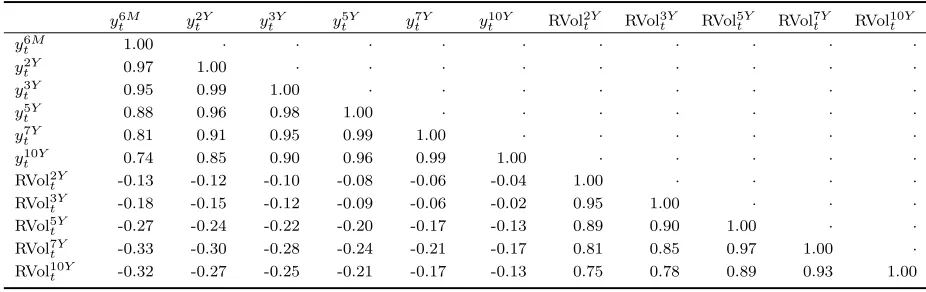
Table 1 reports summary statistics for the zero-coupon yields (panel A), realized and implied volatilities (panel B), and unconditional correlations between yields and realized volatilities, as well as realized and implied volatilities (panel C).
Factors in volatilities. The principal component analysis suggest that, similar to yield levels,
also realized yield volatilities can be described by three factors. The first three principal components explain 90%, 7% and 1.5% of the realized volatilities with maturities between two- and ten-years. Their loadings resemble the level, slope and curvature and are plotted in Figure 2. The recent financial crisis emphasizes the multivariate structure dynamics of yield volatilities. As seen in panel b of Figure 1, while the two-year realized volatility increased already during the summer 2007, the ten-year volatility remained relatively low until the Lehman collapse. Following the extraordinary measures undertaken by the Fed and the US Treasury, and the promise of low rates for an “extended period of time,” the two-year realized volatility fell sharply in the beginning of 2009, and reached all-time low in the second half of 2010. At the same time, the ten-year volatility remained at elevated levels, perhaps coinciding with the uncertainty about the long-term economic outlook.
Link between interest rates and volatilities. Much of the theoretical and empirical evidence points to a link between the level of interest rates and their volatility. Affine or quadratic models, for instance, imply that the same subset of factors determines both yields and their volatilities. As one example, a single-factor CIR model suggests that the volatility is high whenever the short rate is high (Cox, Ingersoll, and Ross, 1985). While the
7MOVE is a weighted index of implied volatilities of one-month options on Treasury bonds. The maturities
CIR-type prediction remained valid through the early 1980s (Chan, Karolyi, Longstaff, and Sanders, 1992), more recently the unspanned stochastic volatility (USV) literature has argued that the yield-volatility relation is weak (Collin-Dufresne and Goldstein, 2002; Andersen and Benzoni, 2010). Using realized volatility we find that this relationship can in fact be nonlinear.8 The shape of a nonparametric regression fitted to the data suggests a slightly asymmetrically U-shaped pattern: volatility is low for intermediate maturities, and increases when rates move toward either extreme, more so when interest rates become low. Naturally, after the short rate reaches the zero lower bound during the recent crisis, the volatility at the short end of the curve also dies out. Outside this special interest rate environment, the rise in volatility is more pronounced in low interest rate regimes than it is in high interest rate regimes. This is reflected in the negative unconditional correlations between yields and volatilities reported in panel C of Table 1.
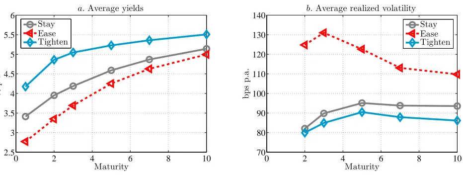
Figure 3 plots average yield and realized volatility curves conditional on the monetary policy stance (easing, tightening or no action).9 A monotonically increasing average term structure of yields is accompanied by a humped term structure of volatilities, with the hump most pronounced at the three-year maturity during easing episodes. In our sample, a monetary policy easing is associated with a rising slope of the yield curve, a higher level of yield volatility and an increased magnitude of the volatility hump.
Implied vs realized volatilities. Table 1shows that on average, and most visibly at the short
maturity, implied volatilities exceed realized volatilities, suggesting a negative volatility risk premium. For the two- and five-year maturity, the difference between the implied and real-ized yield volatilities is about 22 and 14 basis points, respectively. Relative to the realreal-ized volatilities, implied volatilities are more persistent and have a lower unconditional standard deviation. The bottom panel of Table1reports unconditional correlations between realized and implied volatilities and the MOVE index. The lowest correlation reaches 0.51 between the ten-year implied and two-year realized volatility. The correlation between MOVE and our implied volatility series exceeds 0.9, except for the two-year maturity where we cover only a short part of the sample. At the weekly frequency, the three principal components of realized volatilities explain between 45% and 49% of variation in implied volatilities across maturities. Given that there is a lot of high-frequency variation in realized volatilities,
8The results summarized here are not reported in any table for brevity. 9
this share increases to between 68% and 72% when we smooth realized volatilities with a four-week moving average.
II. The model
We propose a no-arbitrage model for the joint dynamics of nominal yields and their time-varying second moments. The model introduces multiple factors in yield volatilities, and allows for priced yield and volatility risks. We use the model to decompose and analyze the variation in the covariance matrix of yields in a way that is consistent with a small number of factors in the term structure, and in particular the components of short rate expectations and the term premia. The model also allows us to study the role of yield volatilities for the cross section of yields and for the bond risk premia.
II.A. The no-arbitrage framework
We distinguish between yield curve factors Xt, and covariance factors Vt. The physical
dynamics are given by the system:
dXt = (µX +KXXt)dt+
p
VtdZX,tP (2)
dVt = (ΩΩ ′
+M Vt+VtM ′
)dt+pVtdWtPQ+Q ′
dWP′ t
p
Vt, (3)
whereXtis an-dimensional vector, andVtis an×n covariance matrix process (Bru, 1991;
Gourieroux, Jasiak, and Sufana, 2009);ZP
X andWPare ann-dimensional vector and an×n
matrix of independent Brownian motions, respectively; µX is a n-vector of parameters and KX, M and Qare n×n parameter matrices.10
We consider a setup in which n = 2, i.e. Xt contains two factors with a time-varying
conditional covariance matrix. Since we do not model the time-varying second moments at the shortest maturity range, we introduce a third yield curve state ft evolving as:
dft = (µf +Kf XXt+Kfft)dt+σfdZf,tP . (4)
Kf and σf are scalars, Kf X is a 1×2 vector, and Zf,tP is a Brownian motion independent of
all other shocks in the economy. As such, Xt can impact the conditional expectation offt
10To ensure a valid covariance matrix process
through the drift. Time-varying volatility enters the model through Vt that describes the
amount of risk in the economy, with off-diagonal elements ofVtdetermining the conditional
covariance between Xt’s. We focus on modeling the stochastic covariance of yields of
intermediate to long maturities, whose variation we can observe with support of high frequency data. Given the different institutional properties of shortest maturity yields and the unavailability of traded high-frequency data, we assume constant conditional volatility for ft.
We collect Xt and ft factors in a vector Yt = (X ′ t, ft)
′
, whose dynamics can be compactly written as:
dYt= (µY +KYYt)dt+ ΣY(Vt)dZtP, (5)
where ΣY(Vt) is a block diagonal matrix with √Vt and σf on the diagonal, and KY = KX 0n×1
Kf X Kf
!
.
The short interest rate is an affine function of Xt and ft:
rt=γ0+γ
′
XXt+γfft=γ0+γ
′
YYt (6)
with γY = (γ ′ X, γf)
′
.
Bonds are priced by no-arbitrage. We specify the stochastic discount factor as:
dξt
ξt
=−rtdt−Λ ′ Y,tdZ
P
t −T r Λ ′ V,tdW
P t
, (7)
with market prices of risk:
ΛY,t = Σ
−1
Y (Vt) λ0Y +λ1YYt
(8)
ΛV,t =
p
Vt
−1
Λ0
V +
p
VtΛ1V. (9)
This specification assumes that shocks to both yield and volatility factors are priced, preserving the tractable affine structure of the model. The market price of risk parameters have the following dimensions: λ0Y,(3×1),λ
1
Y,(3×3), Λ
0
V,(2×2), and Λ
1
V,(2×2). Equation (8) follows
Prices of nominal bonds are obtained by solving Pτ t =E
Q t e
−Rτ
0 rsds. The solution for the
nominal term structure has an affine form:
P(t, τ) = exp{A(τ) +B(τ)′
Yt+T r[C(τ)Vt]}, (10)
whereT r(·) denotes the trace operator. The coefficientsA(τ), B(τ) andC(τ) solve a system of ordinary differential equations:
∂A(τ)
∂τ =B(τ)
′
µQY +1 2B
2
f(τ)σf2 +T r
ΩQΩQC(τ)
−γ0 (11)
∂B(τ) ∂τ =K
Q′
Y B(τ)−γY (12)
∂C(τ) ∂τ =
1
2BX(τ)BX(τ)
′
+C(τ)MQ+MQ′
C(τ) + 2C(τ)Q′
QC(τ), (13)
where KYQ, MQ and ΩQ are the parameters of the risk neutral dynamics. We split the
B(τ) loadings as B(τ) = [BX(τ) ′
, Bf(τ)] ′
. The boundary conditions for the system (11)– (13) are A(0) = 01×1, B(0) = 03×1 and C(0) = 02×2. B(τ) has a standard solution as in
Gaussian models; C(τ) solves a matrix Riccati equation. All technical details are collected in Appendix II.
Defining yτ
t =−τ1lnP τ
t, the term structure of interest rates is obtained as:
ytτ =−1
τ{[A(τ)−B(τ)
′
Yt−T r[C(τ)Vt]}. (14)
The instantaneous yield covariation is only driven by the covariance factors, Vt:
vτi,τj
t :=
1 dthdy
τi t , dy
τj t i
= 1
τiτj{
T r{[BX(τi)BX(τj) ′
+ 4C(τi)Q ′
QC(τj)]Vt}+Bf(τi)Bf(τj)σf2}, (15)
and the conditional risk-neutral expectation of the annualized yield variance over horizon h is:
vQ,τt,t+h =EtQ
Z h
0
vτt+sds, (16)
The model implies that the instantaneous expected return, brpτ
t, to holding a bond with
maturity τ is:
brpτt = λ0Y +λ1YYt
′
B(τ) + 2T r(Λ0V + Λ1VVt)QC(τ)
. (17)
The first term in (17) is common with the Gaussian dynamic term structure models (DTSMs), the second term is a new element that captures the effect of volatility on the bond risk premia. Thus, volatility states are allowed to affect both the levels of yields in equation (14) and the bond risk premia in (17). The variance risk premium, defined as the difference between the expected h-period variance under the physical and risk neutral dynamics:
vrpτt,t+h =vt,tQ,τ+h−vt,tP,τ+h (18)
is determined by the volatility statesVtand the corresponding market price of risk
param-eters in equation (9).
II.B. Discussion
Our distinction between volatility and yield curve states builds on the Am(n) classification
of ATSMs introduced by Dai and Singleton (2000). The new element is that Vt represents
a covariance matrix, involving an interaction factor which can change sign.11 The form of
Vt leads to a three-factor model for the second moments of yields with two volatility and a
covariance state. This structure helps us to overcome the difficulties of DTSMs in matching conditional volatilities of long-maturity yields reported in the literature. The combination of six factors gives the model the flexibility to fit both yields and volatilities. The state space we consider is large, but involves a relatively small number of identified parameters (13), excluding the market price of risk parameters in (8)–(9).
The presence ofVtin expression (14) distinguishes our model from the unspanned stochastic
volatility settings, which impose explicit restrictions so that the volatility factors do not enter the cross section of yields. Such separation usually improves the volatility fit of low-dimensional ATSMs (Collin-Dufresne, Goldstein, and Jones, 2009). However, as highlighted by the literature, there appear to be few reasons, except statistical ones, for such constraint to strictly hold (Joslin, 2007). The volatility variables could appear in the term structure of
11
yields through at least two channels. One of them is the convexity (e.g. Phoa, 1997). The second one is the effect that volatility has on the risk premia. We explore the importance of these channels below.
II.C. Estimation
We estimate the model on a weekly frequency (∆t = 521) combining pseudo-maximum likelihood with filtering. All technical details on the estimation and identification are presented in Appendix III.A.
We introduce three types of measurements for yields (˜yτ
t), their quadratic covariation (˜v τi,τj t )
and the expected risk neutral variance over the next month (˜vt,tQ,τ+4):
˜
ytτ =f1(Yt, Vt; Θ) +
p
R1e1,t (19)
˜ vτi,τj
t =f2(Vt; Θ) +
p
R2e2,t (20)
˜
vQ,τt,t+4 =f3(Vt; Θ) +
p
R3e3,t. (21)
Functions fi(·), i = {1,2,3} denote the model-implied expressions corresponding to the
measurements; Θ collects model parameters. ˜vτi,τj
t is obtained from the high-frequency
zero-coupon yield curve using the realized covariance estimator (1). The expected risk neutral variance vQ,τt,t+4 is identified from the squared implied volatility series.
We assume additive, normally distributed measurement errors ei, i = {1,2,3} with zero
mean and a constant covariance matrix. In estimation, we use six yield measurements with maturities of six months and two, three, five, seven and ten years withR1 =σ2yI(6×6), where
I(6×6) is an identity matrix, and σy is common across maturities. We include four realized
variance measurements: realized variances of the two-, five- and ten-year bond and the covariance between the five- and ten-year bond, as well as three measurements for the risk neutral variance with underlying bond maturities of two, five and ten years. The two-year implied volatility is available only in part of the sample, therefore in estimation we treat the initial observations as missing. Since our implied volatility series have coupon bonds as the underlying, we use the average duration of the bond during our sample period to obtain the zero-coupon implied volatility equivalent. The implied volatility measurements are therefore matched with the model-based risk neutral volatility vt,tQ,τ+4 with τ = 1.9, 4.4 and 7.5 years, respectively.12 In total, we have seven variance measurements, and for each
12
we allow a different measurement error, i.e. R2 and R3 are diagonal matrices with four and three parameters, respectively.
In order to handle the non-Gaussianity in factor dynamics we use the square-root Unscented Kalman Filter (UKF), proposed by Julier and Uhlmann (1997).13 We maximize the likelihood with the global optimization algorithm of Price, Storn, and Lampinen (2005).
Finally, we impose parameter restrictions that ensure econometric identification of the model. After that, the baseline model has 13 parameters which drive the yield curve (six of which describe the market prices of risk), and ten parameters which drive the volatilities (four of which describe the market price of risk).
III. Empirical results
This section uses the model to analyze the empirical properties of interest rate volatility. First, we discuss a decomposition of volatility into a short rate expectations component and a term premium component. Second, we study how volatility affects the yield curve and the level the bond risk premia.
III.A. Estimated factors
The model fits the data well indicating that it has the flexibility to summarize information in yields, and in realized and implied volatilities. A summary of the model’s performance is provided in Appendix IV.
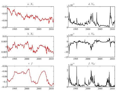
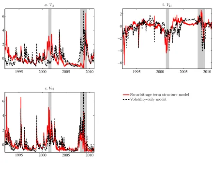
Figure4plots the model-implied factor dynamics. Panels on the left display the evolution of the yield curve factorsY = (X1, X2, f), those on the right show the corresponding volatility states ¯V = (V11, V21, V22),14 capturing the conditional covariance of the yield curve factors X1 and X2.
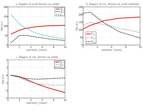
Figure 5 shows how these factors affect the yield curve. Each line presents the model-implied factor loadings in equation (14), scaled by one standard deviation of each factor. Panel adisplays the B(τ) coefficients. The effect of ft is most pronounced at the short end
of the yield curve. The time series of ft in Figure 4suggests that this factor closely traces
13
See e.g. Carr and Wu (2007) and Christoffersen, Jacobs, Karoui, and Mimouni (2009) for the recent applications of the unscented Kalman filter to asset pricing.
14We rotate the yield curve factors such that their increase has a positive effect on the yield curve. In
practice this amounts to multiplyingX2 by−1. Correspondingly, the sign of the covariance state V21
the short-maturity rates: its correlation with the the Fed funds target is 0.96. In that narrow correlation sense, ft reflects the stance of the monetary policy within the model.
The two remaining factors influence the longer segment of the yield curve: the impact of X1 increases with the maturity, while X2 affects most strongly the short-to-intermediate maturities between two and three years.
The volatility factors in panel b behave accordingly: the effect of V11 on interest rate volatility rises whereas that of V22 declines with the maturity. Respectively, we label them as the long-end and the short-end volatility. TheV21term drives the conditional covariance between the yield curve factors. The estimated dynamics suggest that the covariance state changes sign during our sample period.
As visible in the right-hand panels of Figure 4, the estimates of the Vt process imply that
the long- and short-end volatility have different time series properties. Not surprisingly, volatility states are substantially less persistent than the yield curve states. A less imme-diate observation is that the short-end volatility is less persistent than the long-end. The half-lives under the real world (P) dynamics are below one year (47 weeks) for the short-end volatility V22 and above 1.5 years (90 weeks) for the long-end volatilityV11.
III.B. Volatility of term premia versus volatility of short rate expectations
Our factors are latent, and therefore they are not directly linked to any observable macro quantities. However, the structure of the model allows us to analyze the interactions between well-defined economic quantities in the yield curve.
Yield volatility stems from either volatile short rate expectations, or volatile term premia, and comovement between the two (plus a convexity-related term). If interest rates become more volatile, one would like to understand which component contributes to the volatility increase. To the extent that short rate expectations reflect expectations about the future path of monetary policy, their volatility can be informative about the amount of uncertainty surrounding that path at different horizons. The conclusion that we draw from this section is that the model-based volatility factors have separate interpretations in terms of their link to short rate expectations and term premia.
ret,t+τ = 1 τE
P t
Z τ
0 rt+s
ds (22)
rpyτt = 1 τ
EtQ
Z τ
0 rt+s
ds−EtP
Z τ
0 rt+s
ds
, (23)
wherere
t,t+τ denotes the expected average short rate, andrpytτ is the term premium. These
expressions are affine in Vt and have a tractable form provided in Appendix V.
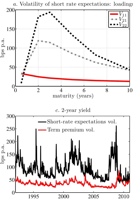
Figure 6 shows how volatility states contribute to the second moments of short rate expectations (panela) and risk premium (panelb) across maturities. The loadings reveal an interesting distinction. The long-end volatility, V11, emerges as the dominant factor for the variance of the term premium, but it has a minimal contribution to the variance of short rate expectations.15 The short-end volatility, V22, does the opposite: While its impact on the term premium part is effectively zero, this factor plays a key role in generating the variance of short rate expectations. It seems justified to label these factors as the term premium and short rate expectations volatility, respectively. Below, we use interchangeably the terms short-end (long-end) volatility and short rate expectations (term premium) volatility. The covariance state contributes to both, but its effect on the short rate expectations component is stronger, suggesting that an increase in the comovement between yields across maturities makes short rate expectations more volatile.
Panels c and d in Figure 6 plot the time series of volatilities of expectations and of term premia for the two-year (panel c) and the ten-year yield (panel d). The volatility of the two-year bond is dominated by the expectations part, while that of the ten-year bond—by the term premium part, even though the volatility of short rate expectations still plays a significant role at the ten-year maturity. This evidence is consistent with a scenario in which short rate expectations are mean reverting, and their effect declines with the maturity, i.e. the Fed has a limited control over the long-end of the yield curve; this is accompanied by an increasing role of the term premium at the longer maturities range.
Given their different interpretation, it is useful to study the behavior of volatility states over the business cycle. Figure 7 displays the evolution of long- and short-end volatility in our sample. Consistent with its link to short rate expectations, the short-end volatility typically rises before recessions, perhaps on an increased uncertainty about an upcoming monetary policy easing; in those episodes the long-end (term premium) volatility remains
15
contained. After recessions both tend to rise. This is the case for each post-recession period in our sample: in 1992 (post 1990–1991 recession) the long-end volatility increased by more than three standard deviations away from its unconditional mean; similarly in 2003 (post 2001 recession) it moved almost four standard deviations from the mean. The short-end volatility factor exceeds the four standard deviations mark five times in our sample all of which concur with monetary policy easings. It also increases during periods of distress in asset markets such as the LTCM, the Russian crisis or the dot-com bubble, which in the 1990s and 2000s have been paired with supportive monetary policy actions. During the recent financial crisis, the short-end volatility reached extreme levels already in the Fall 2007 and persisted until 2009. The long-end volatility, instead, remained low until the bankruptcy of Lehman Brothers, after which it peaked in March 2009. Given its interpretation as the term premium volatility, one could view this as a sign of the bond market being concerned about the consequences of fiscal and non-standard monetary policy measures for the future risk of Treasuries. We provide evidence supporting this intuition in Section IV.
III.C. Comovement between term premia and short rate expectations
From the monetary policy perspective, one important reason for studying the second moments of yields is the question of how short rate expectations and risk premia comove over time. For instance, a negative comovement in an easing environment may suggest that the Fed faces a tradeoff between lowering short term interest rates to stimulate the economy, and increasing the inflation risk premium. By modeling directly the stochastic covariance of risks, our setting is uniquely suited to study the empirical properties of this tradeoff.
Panel ein Figure6displays the role of the model-implied factors in generating the comove-ment between shocks to the term premia and to short rate expectations. To obtain the loadings, we compute the conditional covariance of the two objects in equations (22) and (23). Consistent with its interpretation as the covariance state, the figure shows that the V21 factor has the largest impact on the covariance, which increases upon a positive shock to the factor.
is low on average and positive, with its unconditional mean reaching 0.14 for two-year bond and 0.21 for the ten-year bond. Second, the correlation is persistent but clearly time-varying, changing sign multiple times during our sample. In the plot, we superimpose its dynamics with the Fed funds target (rescaled to fit the graph). On average, the correlation between risk premia and expected short rates increases during easings and declines during tightenings. Interestingly, the model interprets the Greenspan’s conundrum period, i.e. the lack of response of long-term yields to the Fed’s 2004/05 tightening, as a decline in the correlation between the expected short rate and the term premium from nearly one to negative −0.4.
The evolution of the tradeoff between expected short rates and the term premia, along with their low unconditional correlation, casts new light on the view that in the last two decades the link between short- and long-term interest rates has been largely severed (e.g. Thornton, 2012).
III.D. Additional model implications
This section focuses on the channels through which volatility impacts the yield curve. We find that in terms of modeling the cross-section of interest rates, analyzing priced sources of risk in the term structure, and the time-varying bonds risk premia, the conclusions from the model with a rich second moments dynamics are close to these based on a Gaussian setting. At the same time, in Section IV we show that modeling interest rate volatility is not a void exercise, in that volatility states contain information about the economy that cannot be extracted from yields themselves.
III.D.1. Implications for the Treasury risk premia
Expression (17) shows that the model-based bond risk premia have two components loading on the yield curve and volatility states, respectively. Abstracting from the time-varying second moments in Yt, the first component arises similarly in Gaussian models and we will
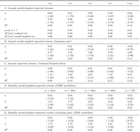
The results are collected in Table 2. We compute the model-implied expected bond excess returns for an annual holding period which is the horizon customarily used in the literature on bond return predictability. We then regress the realized excess returns from the data on the model-implied risk premia. We consider three variants of the regressions. Panel A is based on the total model-implied risk premium; panel B involves only the Gaussian part and zeros out the risk premium variation due to the volatility states. Panel C benchmarks the model-based results to the predictability obtained with the return forecasting factor of Cochrane and Piazzesi (2005, CP). In our sample, the CP factor predicts between 8% and 19% of the variation in the annual realized excess returns at maturities between two and ten years. The model-based risk premium gives a slightly lower degree of predictability ranging between 3% and 13%.16 A comparison of panels A and B of the table suggests that priced volatility risk does not contribute in a significant manner to the predictable variation of bond excess returns.
One may wonder how this conclusion depends on the return horizon that we predict. Given the impersistent nature of yield volatility, one could expect the effect of volatility states on the risk premium to be material only at short horizons. Panel D and E of Table 2 present results analogous to the above regressing the realized returns with a holding period of one month onto the instantaneous model-based risk premium. The results appear to confirm the previous conclusion that the contribution of the priced variance risk to the bond risk premium is minute.
However, the model implies a non-zero variance risk premium: on average, investors pay a premium for the volatility protection. The variance risk premium defined in equation (18) has a slightly humped pattern across maturities, is the highest at the maturity of three years, and declines with maturity. In basis points terms, the model implies the volatility risk premium, measured as the average of
q
vt,tQ,τ+h −
q
vt,tP,τ+h with h = 4 weeks, equal to 21 (22.5) basis points at the two-year (three-year) maturity and less than 9 basis points at the ten-year maturity. In that yield volatility at short maturities is mostly driven by the volatility of short rate expectations, it seems plausible that the variance risk premium
16At longer maturities, the realized excess returns load on the model-based risk premia with a slope
coefficient that exceeds one, suggesting that risk premium from the model is less volatile than the data. The non-unit coefficient may be a consequence of our relatively short sample period. We can reject the non-unit coefficient only for maturities of nine and ten years at the 5% level. Using survey data to measure expected excess bond returns on the two-year bond we also find a non-unit (and insignificant) coefficient and a ¯R2
reflects mainly a compensation for the risk related to volatile expectations about monetary policy.
III.D.2. Role of volatility in the cross-section of yields
A question that has attracted attention is how volatility affects the cross section of inter-est rates. Quantifying this effect requires a model that is rich enough to accommodate the empirical properties of both the first and second moments of yields. The literature summarized in the introduction argues that standard dynamic term structure models lack the flexibility to generate realistic yield volatilities, especially at the long end of the term structure. Therefore, potential misspecification complicates a model-based inference about the linkages between yields and volatilities. Our approach is different in that we equip the model with a multifactor structure that the data calls for but also ask it to actually match the observed second moment dynamics.
Panel c of Figure 5 uses equation (14) to measure how the shape of the term structure changes when the volatility changes. The graph makes clear that this channel is quanti-tatively small. Even a two standard deviation shock to volatilities has a total (negative) impact on the ten-year yield of about eight basis points. It is almost entirely driven by the long-end (term premium) volatility state and, consistent with the usual convexity effect, most visible at long maturities. Interestingly, we find that the short-end volatility related to short rate expectations is essentially impossible to uncover from the cross-section of yields: Its corresponding yield-curve loadings are effectively zero. As such, using terminology of Duffee (2011), this factor can be interpreted as hidden. In contrast to the USV models, this result is obtained without imposing constraints on the model parameters that would prevent a priori the volatility states from entering the cross section of yields.
III.E. Comparison with a volatility-only model
is below 0.3. This suggests that the no-arbitrage restrictions are useful in disentangling the volatility of short rate expectations from the volatility of the risk premia. The stronger correlation of the short-end volatility is consistent with short rate expectations driving a higher share of the overall volatility in yields. Figure 9 shows that the largest differences between factors implied by these two settings arise during recessions. While the short-and long-end volatility factors from the no-arbitrage model increase in different recession phases, the factors in the volatility-only model move much more in sync during downturns. For comparison, Table3also reports correlations with the first three principal components of the realized and implied yield volatilities. The volatility states from the no-arbitrage model have a significantly weaker relationship to the principal components than those from the volatility-only model.
IV. A macro-finance link
This section verifies our interpretation of yield volatility factors by linking them to observ-able uncertainty proxies. We also show that interest rate volatility, and in particular the volatility of short rate expectations, provides new information about the economy that is not contained in the standard yield curve factors.
IV.A. Macroeconomic uncertainty
We relate volatility factors from the model to survey-based proxies for expectations and uncertainties about the macroeconomy. Forecasts of macro variables are from the Blue Chip Financial Forecasts (BCFF). As documented in the transcripts of the FOMC meetings, these surveys are regularly used by policymakers at the Fed to read market expectations.17 AppendixI.Fprovides details about the survey data including their timing within a month. We use responses of individual panelists to construct proxies for the consensus forecast and for the uncertainty. Each month, the consensus is computed as the median survey reply. Uncertainty is measured with the mean absolute deviation of individual forecasts.18 We consider forecasts of the real GDP growth (RGDP), the federal funds rate (FFR) and all-items CPI inflation (CPI). For each variable and each month we have a term structure
17
Between 1994 and 2007, the FOMC transcripts refer to the forecasts from the Blue Chip survey 146 times during 61 FOMC meetings.
18Disagreement in survey forecasts could be more reflective of differences of opinions rather than
of forecasts from the current quarter out to four quarters ahead. To summarize this information, we compute the average consensus/uncertainty across horizons. We also relate yield volatility to the economic policy uncertainty index constructed by Baker, Bloom, and Davis (2013, BBD).
We run contemporaneous regressions of model-based volatility states on the above variables. Since consensus forecasts can be very persistent, given our relatively short sample, we use their monthly changes rather than levels. Table4summarizes the results for the 1992–2010 sample (panel A), and for the 1992–2007 sample excluding the recent crisis (panel B). For the full sample, we capture between 38% and 42% of variation in the yield volatility states and about 14% in the covariance state. These shares remain similar in the 1992–2007 sample. The three volatility states differ in the way they load on the explanatory variables. In terms of macro consensus, the long-end volatility is positively related to the changes in the expected RGDP. This link is most visible during the recent crisis, where the long-end volatility factor peaked after growth expectations started to recover from the bottom of the recession.19 One interpretation of the positive sign is that despite the initial signals of recovery, the long-end volatility has moved up on concerns about long-term consequences of the fiscal and monetary stimulus. The model associates this pattern with an increased volatility of the term premia. We find support for this interpretation based on the policy uncertainty index below. The short-end volatility, instead, comoves negatively with changes in the monetary policy measured with the FFR. A 50 basis points negative change in the expected FFR raises the short-end volatility by approximately a half standard deviation.
Both short- and long-end volatility increase with the uncertainty about the real economy. The most important difference between them is that the short-end volatility comoves positively with the level of uncertainty about the FFR, while the long-end volatility— with the economic policy uncertainty as measured with the BBD index. This distinction aligns well the interpretation of these factors as the volatility of short rate expectations and term premia, respectively. It is also interesting in the context of the findings of BBD, who argue that their index reflects mainly uncertainties about taxes, spending as well as monetary and regulatory policies. In particular, they find that since 2008 the increases of the index have been dominated by the elevated tax, spending and regulatory concerns, but not concerns about the Fed. This is supported with the behavior of the yield volatility
19
states just before and during the crisis (see Figure 7): The short-end volatility increased already in 2007 and then declined ahead of the long-end volatility, while the latter remained low until mid-2008, rose afterwards and remained high through the end of our sample in 2010. A projection of the policy uncertainty index on the volatility states (not reported in any table for brevity) reveals that the index covaries most strongly with the short-end volatility before the crisis, and with the long-end volatility from 2007 onwards. Thus, the behavior of the model-based volatility factors and their respective links to the Fed and to the economic policy uncertainties suggest that these factors distill and trace consistently over time particular types of risk.
It is worth noting that the covariance state has the weakest relation to the survey-based consensus and uncertainty measures. To the extent that it drives the comovement between the term premium and short rate expectations, linear regressions like the ones we estimate above may not be appropriate to capture the information this factor contains. However, we find that covariances between realized macro variables and interactions between survey-based uncertainty measures are able to explain up to 33% of its dynamics, with the interaction of uncertainty about the FFR and the CPI being the most significant one.
IV.B. Forecasting growth
The literature has documented that the slope of the yield curve has predictive power for the economic activity: a higher slope predicts an increase in the real activity, consumption and investment at horizons between one and two years ahead (Estrella and Hardouvelis, 1991; Harvey, 1989). We show that there is additional information in yield volatility over and above that contained in the cross section of yields.
We forecast economic activity, measured with the CFNAI (Chicago Fed National Activity Index)20 by estimating the following regression:
CFNAIt+k=β ′
kXt+εt+k, k ={0,1, . . . ,24} months, (24)
20The CFNAI is published on the Chicago Fed web page as a weighted average of 85 existing monthly
where as explanatory variables inXtwe consider yield curve factors (principal components),
and/or volatility states. We predict activity at horizons ranging from the current month through 24 months ahead.
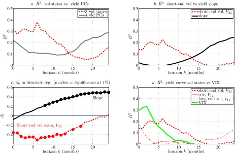
Figure8shows the results for different specifications of equation (24). Panelacompares the predictive ¯R2obtained from two regressions using as the explanatory variables: (i) the three volatility states obtained from the model, and (ii) the first four yield PCs. The figure reveals different predictability patterns in the two specifications. While in volatility regressions the highest ¯R2s are obtained at short horizons reaching a peak of 37% at k = 7 months, the yield PCs regressions give initially low predictability which increases at horizons above one year, and reaches 29% at k= 24.
In panelb, we repeat the same predictive exercise but using only the short-end volatilityV22 and the yield curve slope. We find that these two variables account for the main part of the predictability in the previous regressions. The predictive power of the short-end volatility is the highest at k = 7 months with ¯R2 of 23%. The slope-only regression, instead, gives the maximum predictability at horizons above one year, which is in line with the evidence in the literature, e.g. at k = 24 the ¯R2 is 25%. In both cases, the regression coefficient is significant at the 1% level.
Panelcsummarizes bivariate regressions with slope and short-end volatility included jointly. In the plot, we mark horizons for which each regressor is significant at the 1% level. The pattern of coefficients is consistent with the previous graphs suggesting that yield volatility operates at shorter horizons than the slope. Importantly, for all specifications, the short-end volatility has a negative coefficient. Using implications of our model, a rising volatility of short rate expectations is a signal for lower growth several months ahead.
Panel d compares the properties of the three volatility factors from our model in terms of forecasting growth, and shows that the short-end volatility dominates the other two factors. The covariance state does not predict activity at all, and the long-end volatility is significant (with a negative coefficient) only in contemporaneous regressions (k = 0) and at the long horizon, although we find that this latter result is not robust to the exclusion of the crisis years.
volatility is different than that in the VIX. In bivariate regressions (details not reported), both VIX and the short-end volatility remain significant at the 5% level for k up to about nine months (VIX) and one year (V22), and both preserve their negative coefficients.
The forecasting power of the short-end volatility and the slope remains robust to the exclusion of the crisis years. In the pre-crisis sample, the short-end volatility captures up to 17% of variation in the future CFNAI at short horizons. At the same time, with the exclusion of the crisis, the predictive power of VIX becomes significantly weaker.
IV.C. Liquidity measures
Liquidity and the highest quality of collateral are important motives driving demand for the US Treasuries (Krishnamurthy and Vissing-Jorgensen, 2010; Longstaff, 2004). We ask how these motives are related to yield volatility. These results are summarized in Table 5.
We consider several liquidity measures that have been proposed in the literature and which capture multifaceted nature of liquidity. First, we use the Hu, Pan, and Wang (2012, HPW) noise illiquidity, which measures temporary price deviations of Treasury bonds from a smooth yield curve. HPW show that the illiquidity is related to the availability of arbitrage capital in the market. An increase in illiquidity signals that arbitrage capital becomes scarce and the overall market liquidity deteriorates.
As a second measure, we consider the systematic liquidity factor in the equity market from Pastor and Stambaugh (2003, PS). A lower value of the PS factor indicates a worsening equity market-wide liquidity.
Third, we use the value funding liquidity proposed by Fontaine and Garcia (2012, FG), and filtered from on- and off-the-run Treasury bonds. An increase in the value of funding liquidity is interpreted as a tightening of funding conditions.
Our fourth measure, labeled “Fails,” is the total monthly par value of transaction (in logarithm) that involve failures to deliver a Treasury bond needed to settled a trade.21 In periods of a large demand for liquid collateral, market participants may choose to fail to deliver on their repo transaction.22 As increase in the volume of fails should then be
21
The data on fails is available from the website of the New York Fed. Alternatively, we could use the variation in haircuts applied to Treasury collateral to study the collateral channel—an increase in Treasury volatility lead to an increase in haircuts applied to Treasury collateral which trigger margin calls and thus decrease the liquidity in the market. Due to the lack of data on haircuts we analyze only the failures to deliver.
22
informative about the demand pressure in the Treasury market, and the value of liquid collateral.
Finally, as a fifth variable, we consider the TED spread, i.e. the spread between the three-month LIBOR and the three-three-month T-bill rate. An increase in the spread is interpreted as a sign of rising credit risk in the banking system and thus tightening of credit provision to the economy.
Panel A of Table 5 presents contemporaneous regressions of each of the above liquidity proxies on the three volatility states obtained from the model. Endogeneity is a usual worry in such regression, so our results are merely a statement about the strength and direction of various correlations. We run regressions in levels and in monthly changes. For easy comparison of the coefficients all left- and right-hand side variables are standardized. The regressions reveal a significant link between interest rate volatility and liquidity. While each of the model-implied volatility states differs in terms of economic interpretation and macro variables with which it correlates, liquidity is significantly related to all of them. In general, an increasing yield volatility is associated with deteriorating liquidity conditions. The liquidity measures differ in the strength with which they load on the long- versus short-end volatility and the covariance state. With the exception of the FG factor, the financial crisis is an important event that strengthens the liquidity-volatility link, but this link also exists and is economically strong in the pre-crisis period. In rows labeled “ ¯R2 (92-07),” we report the ¯R2 for the sample ending in December 2007.
We find that the three volatility states capture about 10% of variation in the monthly changes of HPW noise illiquidity. This relationship is stronger than the one found by Hu, Pan, and Wang (2012) for reasons that can be explained with the way we construct the volatility states: First, our volatility factors summarize content of derivatives and the realized variances obtained from high frequency data; second, they aggregate volatility information across different bond maturities.23 Interestingly, we find a pronounced negative relationship between changes in the short-end yield volatility and the PS factor: A dete-riorating equity market liquidity is associated with a simultaneous rise in the volatility of short rate expectations (t-statistics of−6.35). Before the crisis we observe a strong negative contemporaneous link between the level of the FG factor and yield volatility: To the extent
introduced, failures to deliver decreased to extremely low levels. See Garbade, Keane, Logan, Stokes, and Wolgemuth (2010) for more details.
23Hu, Pan, and Wang (2012) measure interest rate volatility as the return volatility of a five year bond
computed with the 21 rolling window. They find a positive but insignificant relationship between monthly changes in volatility and monthly changes noise illiquidity with ¯R2
that the value of funding liquidity comoves with the actions of the Fed (empirically the FG factor decreases during easings when volatility is high), the negative sign is intuitive. The inclusion of the crisis years weakens this connection. Both the volume of fails and the TED spread increase together with yield volatility.
In panel B we study leads and lags between long- and short-end volatility factors and three liquidity measures: PS, HPW and FG. Panel B1 shows regressions when volatility is predicted with lagged liquidity, panel B2 considers the opposite case. Leads and lags are from one through 18 months. To be concise, we only report the coefficients, t-statistics and ¯R2 for the lead/lag with the highest ¯R2. The general conclusion from the table is that liquidity conditions forecast the long-end volatility at horizons above six months. The PS liquidity is significant at a lag of about one year with a negative sign, suggesting that a worsening liquidity in the equities market today forecasts a higher risk premium volatility of Treasuries in the future. Even though predictive regressions do not justify causal statements, this correlation would be consistent with a story in which the Fed supports the equity market through easier monetary policy trading off a higher risk of long-term Treasuries in the future. Similarly, the HPW factor predicts long-end volatility (with a positive and highly significant coefficient) at horizon of about six months. At the same time, the forecasting power of liquidity for the short-end volatility is much weaker. Rather, increasingly volatile short rate expectations anticipate declining liquidity conditions at horizons of about half a year; but the short-end volatility itself does not appear easy to forecast with lags of the liquidity proxies beyond horizons of one or two months.
V. Conclusions
References
Adrian, T., and H. Wu (2009): “The Term Structure of Inflation Expectations,” Working
Paper, Federal Reserve Bank of New York.
Andersen, T. G., and L. Benzoni(2010): “Do Bonds Span Volatility Risk in the US Treasury
Market? A Specification Test for Affine Term Structure Models,” Journal of Finance, 65, 603–655.
Andersen, T. G., T. Bollerslev, F. X. Diebold, and C. Vega(2007): “Real-Time Price
Discovery in Global Stock, Bond and Foreign Exchange Markets,” Journal of International Economics, 73, 251–277.
Ang, A., J. Boivin, S. Dong, and R. Loo-Kung (2010): “Monetary Policy Shifts and the
Term Structure,”Review of Economic Studies, forthcoming.
Baker, S. R., N. Bloom, and S. J. Davis(2013): “Measuring Economic Policy Uncertainty,”
Working paper, Stanford University and University of Chicago.
Barndorff-Nielsen, O. E., and N. Shephard (2004): “Econometric Analysis of Realised
Covariation: High Frequency Based Covariance, Regression and Correlation in Financial
Economics,” Econometrica, 72, 885–925.
Bekker, P. A., and K. E. Bouwman (2009): “Risk-free Interest Rates Driven by Capital
Market Returns,” Working paper, University of Groningen and Erasmus University Rotterdam.
Bru, M.-F.(1991): “Wishart Processes,” Journal of Theoretical Probability, 4, 725–751.
Campbell, J. Y., A. Sunderam, and L. M. Viceira (2013): “Inflation Bets or Deflation
Hedges? The Changing Risk of Nominal Bonds,” Working paper, Harvard Business School.
Carr, P., and L. Wu(2006): “A Tale of Two Indices,” Journal of Derivatives, pp. 13–29.
(2007): “Stochastic Skew in Currency Options,” Journal of Financial Economics, 86, 213–247.
Chan, K. C., G. A. Karolyi, F. A. Longstaff, and A. B. Sanders(1992): “An Empirical
Comparison of Alternative Models of the Short-Term Interest Rate,” Journal of Finance, 47, 1209–1227.
Christoffersen, P., K. Jacobs, L. Karoui, and K. Mimouni(2009): “Non-Linear Filtering
in Affine Term Structure Models: Evidence from the Term Structure of Swap Rates,” Working
Cochrane, J. H., and M. Piazzesi(2005): “Bond Risk Premia,”American Economic Review, 95, 138–160.
Collin-Dufresne, P., and R. S. Goldstein (2002): “Do Bonds Span the Fixed Income
Markets? Theory and Evidence for the Unspanned Stochastic Volatility,” Journal of Finance, 58, 1685–1730.
Collin-Dufresne, P., R. S. Goldstein, and C. S. Jones (2009): “Can Interest Rate
Volatility Be Extracted from the Cross-Section of Bond Yields?,” Journal of Financial Economics, 94, 47–66.
Cox, J. C., J. E. Ingersoll, and S. A. Ross (1985): “A Theory of the Term Structure of
Interest Rates,”Econometrica, 53, 373–384.
Dai, Q., and K. Singleton(2000): “Specification Analysis of Affine Term Structure Models,”
Journal of Finance, 55, 1943–1978.
Diether, K., C. Malloy, and A. Scherbina(2002): “Differences in Opinion and the
Cross-Section of Stock Returns,”Journal of Finance, 57, p. 2113 – 2141.
Duffee, G. R.(2002): “Term Premia and Interest Rate Forecasts in Affine Models,” Journal of Finance, 57, 405–443.
(2011): “Information in (and Not in) the Term Structure,”Review of Financial Studies, 24, 2895–2934.
Estrella, A., and G. A. Hardouvelis(1991): “The Term Structure as a Predictor of Real
Economic Activity,”Journal of Finance, 46, 555–576.
Fisher, M., D. Nychka, and D. Zervos(1994): “Fitting the Term Structure of Interest Rates
with Smoothing Splines,” Working paper, Federal Reserve and North Carolina State University.
Fleming, M. J. (1997): “The Round-the-Clock Market for U.S. Treasury Securities,” FRBNY Economic Policy Review.
Fleming, M. J., and B. Mizrach (2009): “The Microstructure of a U.S. Treasury ECN:
The BrokerTec Platform,” Working paper, Federal Reserve Bank of New York and Rutgers
University.