Nonlinear Programming Algorithms for CAD Systems of
Line Structure Routing
Valery I. Struchenkov
Moscow State University of Radio Engineering, Electronics and Automation, Moscow, Russia *Corresponding Author: [email protected]
Copyright © 2014 Horizon Research Publishing All rights reserved
Abstract Under study is an optimization problem which
arises in line structure routing. In large systems we must solve such problems many times with different source data. So it is necessary to develop non-standard algorithms with using the features of the particular application. The article deals with this kind of algorithms based on the use of constraints features, which arise in the problems of optimal line structures routing. This is a big dimension problem of nonlinear programming. Nonlinear programming problems with the number of variables and constraints in a few hundreds and more demands a lot of machine time.Keywords System of Constraints, Reduced Antigradient,
Basis of Linear Space, Null Space of a Matrix1. Introduction
Many of applied optimization problems can be reduced to finding the plane curve, which meets conditions of smoothness and some other requirements, and for which appropriate quantitative criterion of optimality has a minimum value . In other words, the unknown smooth curve should be the extremal of given functional. When the discrete representation of the desired curve by coordinates of a finite set of points is sufficient, the problem reduces to finding the ordinates at given points. These ordinates are the variables of the problem. Smoothness conditions are expressed as inequalities in ordinates and their differences, and the functional becomes the objective function of many variables. It is required to find a set of variables (an unknown vector z), which satisfies all the constraints and gives minimum of the objective function. Thus, instead of the original variational problem the nonlinear programming (hereinafter NLP) problem is obtained.
Likewise were constructed mathematical models of various problems that arise when designing routes of linear structures [1]. So when designing the optimal longitudinal profile the objective function is the construction cost or building - operating costs [2,3,4,5]. All constraints in this
problem is formalized as a system of linear inequalities [1,2] With the discrete representation of the unknown extremal ( the project line ) with sufficient for practical purposes accuracy we obtain the optimization problem with a few hundred variables and several thousands of constraints – inequalities. This problem is necessary to solve many times with the refinement and detail parameters of the mathematical model because of the interrelation with other design problems [2,4,5 ]. For that reason, the question arises about how to obtain solutions in reasonable time. The standard NLP algorithms was developed for linear constraints of general form. They require too much time in solving problems of large dimension and therefore unsuitable for use in CAD. Therefore still valid implementation of mathematical methods of nonlinear programming in more efficient algorithms and programs was taken into account the peculiarities of a particular task.
The purpose of this article is to demonstrate such capabilities with respect to linear constraints of a special type, arising in computer design of the longitudinal profile of linear structures in the new CAD.
2. Mathematical Model
Denote the unknown broken line z(s) and the coordinates of its nodes (si,zi) (i=1,2,…,n).
The objective function F(z) is convex and has continuous partial derivatives. Her antigradient is denoted f(z). Mathematical models of the objective function discussed in detail in [4,5].
Matrix of the system of linear constraints is denoted by А0. Then we obtain the NLP problem :min F(z) with
(1)
Given matrix A0 and the vector b0 form a valid search area.
All constraints are divided into three groups. 1 On the slopes of the profile elements
. Here (i=1,2,…,n-1).
This limitation is a discrete analogue constraint on first ≤
0 0 A z b
1
(
) /
i i i i i
derivatives.
2On the difference between slopes of adjacent elements (curvature):
(i=1,2,…,n-1). 3 On the ordinates at certain points
or .
These constraints hereinafter are called altitude constraints.
In the general case, the matrix of linear constraints has the form:
Block Af comply with the constraints of the first group. This is two diagonal matrix with elements minus 1 and 1.
Constraints of the second group corresponds to block As - three diagonal matrix. Nonzero elements of the i-th row are: (as) i i=1/∆si;
(as) i i+1 =-(1/∆si+1/∆si+1); (as) i i+2 =1/∆si+1 (i=1,2,…n-2).
The matrix А0 contains Аf and As both with a plus sign and a minus sign because the constraints of the first and second groups are bilateral.
Constraints of the third group correspond to block А3 and А4. In each row of А3 all its elements are zero except one, which is equal to 1 (upper constraint). And in each row of А4 the unique nonzero element is equal minus 1 (lower constraint). In each column of А3 and А4 can be only one nonzero element.
3. Standard Methods for Solving the
Problem
The well- known algorithms of nonlinear programming with linear constraints consist of the following steps:
1 Construction of the valid initial approach z0;
2 Calculation of the anti-gradient of the objective function f0;
3 Defining a set of active constraints;
4 Construction of the descent direction p0 in the bounding hyperplane;
5 Checking conditions for termination of accounts and, if they are satisfied then stop else following step; 6 Calculate step λ and a new iterative point and to item
2;
For a convex objective function process terminates in the neighborhood of minimum point. Known algorithms differ in the construction of descent direction [6,7,8].
At iteration number k when moving along the vector pk all active constraints (i.e. are satisfied as equalities) remain active, if one or more of constraints are not excluded from the active set. If the matrix Аk consists of rows original
matrix А0 corresponding to the active constraints at a given iteration, i.e. and required to , it is obvious that . Set of vectors satisfying this condition is called null-space of the matrix [6]. Null space of the matrix Аk is denoted N (Аk ).
If as descent direction we accept the projection p of anti-gradient f, then the standard algorithm requires to solve the systems of linear equations of large dimension. The duration of an iteration process for large-scale problems may be unacceptable.
By Rozen formula [6]
(2)
Here E is the identity matrix and A consists of rows original matrix corresponding to the active (at a given iteration) constraints and the icon T denotes transposition. The number of iteration (k) hereinafter is omitted.
If we know basis in N(A), i.e. basic matrix С, then [7 ]
Dimension of CTC is equal to dimension of N(A), which may be much smaller than a number of active constraints.
However, the basis (matrix C) allows finding the descent direction without solving a system of linear equations at all. This is so-called reduced anti-gradient [7 ]
(3) Indeed, the vector , as a linear combination of basis vectors with the coefficients forming the vector CTf. Scalar product
if C fT ≠0.
Consequently, the vector g, which is easily calculated for a known basis, is a descent direction because it makes an acute angle with anti-gradient.
If then or f=0 or f N(A).
In the latter case, there is no descent direction in N(A) and it is necessary to consider the exclusion of constraints from the active set, i.e. an increase of dimension N (A). This issue is discussed below.
If the objective function is convex, as in the considered problem, then f=0 means getting the point of absolute minimum on the boundary of the valid search area. In this case, the current iteration point is the solution of the problem. It turns out that in many applications of nonlinear programming it is very simple to build the basis in the corresponding null-space for any combination of active linear constraints.
This allows to create efficient computational algorithms that run several times faster compared to the known standard algorithms. Optimization method is not changed, but his two main points are implemented on the new by taking into account the specific features of the system of constraints.
We show how this was made for the problem of finding an optimal broken line.
4. New Way of Basis Constructing Using
the System Constraints Features
2 1 1 1
( ) / ( ) /
i i i i i i i i
w ≤ z+ −z+ ∆s+ − z+ −z ∆ ≤s t
max
i i
z
≤
z
mini i
z
≥
z
k k k
A z = b A zk k+1= bk
k k=0
A p
T T -1
p = -(E - A (AA ) A)f
T -1 T
p = C(C C) C f
T
g = CC f
( )
N
∈
g
A
T T T
(g,f) = (CC f,f) = (C f,C f) > 0
T
If some variable zj is not included in any of the active constraints then pj = fj. And if all constraints are inactive, the descent direction coincides with anti-gradient.
Further, if at the k-th iteration the matrix A of the active constraints can be divided into blocks of the form:
then the basis in N (A) may be constructed from the basis
с
1,с
2,…,
с
n1-m1in
N(
A
1) and
d
1,d
2,…,d
n2-m2in
N(
A
2).
Then the following
n
1-m
1+n
2-m
2 vectors form a basis in N(A) are:Each of these vectors has n1+n2 component, but in the first group the first n1 components constitute a basis in N(A1) , and the remaining n2 component are zero, while in the second group the first n2 component zero , and the remaining n1 components form a basis in N(A2). Affiliation all of these vectors to N(A) and their linear independence are obvious.
Any of the vector in N(A) is a linear combination of basis vectors. Therefore we can calculate separately the first n1 components of descent direction p (particularly the anti-gradient projection) using the first m1 rows of A, and after this we can calculate its remaining n2 components , using remaining m2 rows of A.
Suppose that such a partition to the sites of independent construction of the descent direction is fulfilled and proceed directly to the construction of the basis for each of them. In the absence of active altitude constraints this constructing depends on a combination of active constraints on the slopes ( rows of Af or - Af) and constraints on the differences between the slopes (the rows of As and / or - As). If the matrix
A is composed only from rows Af or minus Af, that is, there is a site of maximum or minimum slope from a point with number m to a point with number m + r, then N(A) has dimension equal to one and only one (up to a factor) basis vector c, which all components are equal to 1. Normal f-p
orthogonal to N(Ak), i.e.
. It gives , (i=m,m+1,…,m+r) Geometrically equality of all components of the vector р
indicates that within the considered site the project line must be shifted as a whole along the axis of ordinates. These sites hereinafter are called shifting sites or shifting sections.
The resulting formula for pi is correct and in the case where the site of the extremal slope goes to the site of the
extremal curvature and in the common point of these sites a slope difference has extremal value. In this case only shift along the axis of ordinate does not change the extremal values of the slopes and their differences.
If on the site of extremal curvature from the m-th to m + r -th point the elements of extremal slopes are absent, i.e. the matrix A is composed of rows matrix As and / or - As, then we may remain the vector с in basis , but the dimension N(A) is equal two. It is convenient to take the other two basis vectors с1 and с2.
Vector с1 corresponds to rotation of the project line as a whole with the center at the starting point (m), and с2 - at the endpoint (m + r). When turning the slopes of all elements receives equal increments, the difference between them does not change. Belonging to N(A) and the linear independence of с1 and с2are obvious.
We denote abscissa of the rotation center x0. With the known displacement Δk of some point with abscissa xk ≠x0 displacements of all remaining points Δzi within the section from the m-th to m + r should be calculated by formula
(4) Displacements Δzi are equal to the corresponding components of the basis vector.
If there are no fixed points on the rotation section then we compute two basis vectors, in according to the formula (4). For the first vector k=m, Δk=1, x0=xm+r, and for the second k=m+r, Δk=1, x0=xm.
In the presence of a fixed point its abscissa is equal x0 , k = m, Δk = 1 and the formula (4) gives unique basis vector.
If at the right end of the turning section the difference between the slopes is not extremal , and futher the turning section comes again, then we have three basis vectors, etc.
The borders of the turning sections hereinafter called free points.
The starting and ending points of the each site of the first partition are also called free. Dimension of N (A), i.e. the number of basis vectors is equal to a number of free points minus a number of fixed points (after the elimination of degeneracy) minus a number of shifting sections.
We begin construction of the basis vectors at the starting point and our aim is to have in each of them as many zero components as possible.
In general, the algorithm of constructing the basis vectors in each site of the first partition for an arbitrary combination of shifting and rotation sections, presence and location of fixed points consists of the following items.
1. Zero out all the components of the next basis vector corresponding to the considered site of the first partition.
2. Find shifting sections, free and fixed points.
3. Determine the boundaries of zero sections, if they are, and if necessary eliminate degeneracy. Each zero section generates a fixed point at the end of section to the left of it (if there are points to the left) and in the beginning of the section to the right (if any).
Continuation of the zero section to the left or right side is (f - p,c) = 0
1
m r j j m i
f p
r
+
=
= +
∑
0
0
i
i k
k
x x
z
x x
−
∆ =
∆
possible. For example, after turning section on which there are two fixed points, goes the next turning section with one fixed point. Both sections are zero.
4. Within the zero sections all components of the basis vectors are zero. Zero section gives an extra division of the first partition into smaller parcels. They will be considered consequentially. Such a partition unlike partitioning to the sites of the independent construction of descent direction hereinafter will be called the second partition.
5. Determine a free point at which we can specify the displacement without disturbing the active constraints. This point is denoted by P.
At the first step it is the beginning point. If it belongs to the zero section then we move it to the end of this section. Thus, there are two possibilities: point P is free or point P is fixed. In the latter case P is a beginning point of the turning section, and we move it to the end of this turning section. Note that in this section there are no fixed points (otherwise it is zero section). Position of point P is found. This is the beginning of the shifting section, beginning or the end of the turning section.
6. Specify the displacement of the point P equal to 1, i.e. ΔP=1.
7. At the first step, if the point P is the initial point of the shifting section, then we move it to the begin of the next turning section. Further, if the point P is or has been moved to the begin of the turning section, then there are two possible options:
a) in this section are not fixed points, except maybe its endpoint. In any event the components of the basis vector are calculated by formula (4), assuming that the center of rotation is the end of the section and ΔP = 1. Construction of the basis vector in the site of the first partition is completed.
b) there is a fixed point within this section. In this case the fixed point is the center of rotation. The formula (4), with the displacement at the starting point ΔP=1 allows to calculate all relevant components of the basis vector within the rotating section, including the displacement Δ at the its endpoint. The point P is moved to the end of the turning section and
. This is the old situation, but with the new position of the point P and the new ΔP. We move to right a similar manner up to meeting with a turning section, inside which there are no fixed points (variant a) or up to the end of the section of the second ( or the first) partition.
If at the first step the point P has been moved to the end of the turning section due to a fixed point at the its beginning, then it is necessary to additionally calculate the components of the basis vector within this rotating section, using formula (4). The center of rotation coincides with the beginning of the turning section, and at its end ΔP=1.
Constructing of the next basis vector we must begin from the point where constructing of the previous basis vector is ended when moving to the right. Displacement this point is set to 1, and the basis vector is constructed similarly by the motion to right up to zero displacement or the end of the second ( or first) partition. After this we must move to left by
the same rules. If the constructing of the next vector was completed by zero displacement at the endpoint of the site of the first partition, and it is not fixed, then the last basis vector is constructed by specifying the displacement of this point equal to 1. After this we shall move to left by the same rules up to the zero displacement.
Futher, we must consider the next section of the second partition (if it exists), that is, from the end of the previous zero section up to the next zero section or if it absent up to the endpoint of the site of the first partition.
In the absence or exhaustion of zero sections we get the basis corresponding to the site of the first partition, that is to the site of an independent construction of the descent direction. The linear independence of these vectors is guaranteed because the construction of each next basis vector begins with assigning the value 1 to one of his component. At all other vectors this component remains equal zero.
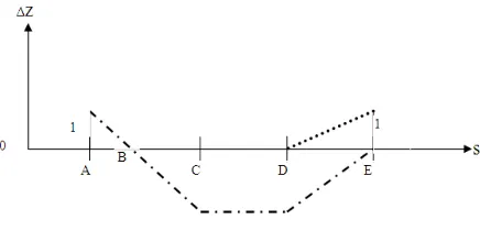
[image:4.595.324.542.335.440.2]An example of displacements corresponding to the basis vectors is shown in Figure 1. AC and DE-rotating sections, CD-shifting section. A, C, D, E - free points, B-fixed point.
Figure 1. An example of constructing the basis vectors
Next, we have two options.
1. Optimize the site of the first partition independently of the others until his extreme point will not be included in some active constraint or descent direction (for example, the anti-gradient projection) will not become zero. In the first case it is necessary to consider a new site with the new system of active constraints. In the second case, we can go to next independent site. 2. Calculate the descent direction for all other sites of the
first partition and optimize the current project line as a whole.
5. New Way of Modification of the
Active Set
An important issue is the modification of the active set through removing from it the constraints that will not be violated at the next iteration. For the linear constraints of the general form this question requires to solve a system of linear equations with the same matrix as in constructing of the antigradient projection. At the each iteration we can remove only one constraint if their system is not simplified to such an extent that each constraint corresponds only to one variable.
P
The presented algorithm for constructing of reduced antigradient does not require the complicated calculations, so the question of removing constraints can be solved by complete enumeration of the active constraints.
At first we construct the descent direction without first constraint, then we check this constraint is violated under the motion along found direction or no. If no, then we use this direction and at the next iteration this constraint is not active. If this constraint is violated, then we check the next one, etc.
However, in our problem there is a possibility of another solution to the question about removing the constraints from the active set. Enumeration of the active constraints remains, but instead of construction a new descent direction for each of them we use a different way to test this possibility.
Rewrite (3) for the reduced antigradient as:
(5)
where ci - basis vectors, q - their number. To test the possibility of removing from the active set the certain constraint with number j, we consider a new vector cq +1, satisfying the following conditions:
for all i=1,2,…,n-m, except i=j.
. Here ai – i-th row of the matrix of active constraints A.
Vector , and therefore it can’t be a linear combination of the old basis vectors and, therefore, does not depend on them.
In other words, with moving off the point zk in the direction cq+1 all active constraints remain active, except the j-th, which is violated.
An additional term (cq+1,f) cq+1 in equation (5) for the new antigradient appears in the new basis (with the added vector
cq+1).
If the new reduced antigradient can be used as the descent direction. For sufficiently small step in this direction j-th constraint is removed from the active set, and all other active constraints remain active. Therefore (cq+1,f)<0 is a condition of removing j-th constraint from the active set. Characteristic that we can remove simultaneously all constraint to which new basis vectors satisfying the conditions 1 and 2, give a negative scalar product when multiplied on anti-gradient.
To construct a new basis vector we should determine to which section (zero, shifting or rotating) the corresponding constraint belongs , and then determine the type of section obtained after its removing, and to construct a vector that violates this and only this constraint.
For example, there is a zero section. We check the removing of altitude constraint and after its removing zero section turns into a shifting section. Then the new basis vector has all the relevant components equal to 1 if we check an upper constraint and minus 1 otherwise. This same vector can be used, if after removing the altitude constraint we receive the rotating section without fixed point. If there is fixed point, then the new basis vector corresponds rotation
with center at this point, etc.
Verifying the possibility of removing one of constraints from the active set can be performed not only in the absence of the descent direction, but at each iteration for an early exit the current point on the of the linear boundary manifold, which owns the minimum point.
6. Practical Application
The system of constraints features are used only for finding the descent direction , including removing of constraints from the active set. Everything else in the standard algorithm: constructing of the initial approach [2,5 ], searching of the step in the descent direction , checking the termination conditions [8], etc. remains unchanged.
The optimal broken line composed of short elements - it is a result only the initial stage of the longitudinal profile designing. This line is usually sufficiently for a quantitative comparison of route options, but for comparison such options which have similar constructing and operating costs and for developing of the final longitudinal profile this line undergoes revision. For this purpose for railway and road designing we use different programs. For railway designing received line is converted to a new broken line, whose elements lengths are not less than the specified values and for road designing it is converted to parabolas or (as an option) to straight and circular curves.
Three computer programs have been developed for such convertion using dynamic programming [9,10]. Finally, at the third stage the received line is subjected to optimization with the simultaneous solution of the other design problems [3,4]. At this stage we use the same software as at first stage, only recounting of derivatives is added [4].
7. The Main Results
Two computer programs have been developed for new CAD of railways routing. The first program implements the gradient projection algorithm, and the second program implements the reduced antigradient algorithm. Both algorithms use the basis vectors, as described above and construct a descent direction for the projected line, varying it as a whole.
The economic effect of optimization the longitudinal profile of roads and other linear structures has been proved in the 70-ies of the last century, in particularly during designing route of the BAM. Due to low computer power at that time we have projected only short sections (up to 5 km)[2]. It corresponds to NLP problem not bigger than 100 variables and 420 constraints. However, even in this case, in the rugged topography was achieved reduction of the construction cost by 7-10% in comparison with the manual designing.
In modern CAD interactive design or simple mathematical i
i i
q
c
f
c
g
( , )1
∑
=
=
1
( ,T ) 0 i q+ = a c
1
( ,T ) 0 j q+ > a c
1 ( )
q+ ∉N
c A
models (mean-square approximation) are used [ 11,12,13 ] . New programs that implement the described algorithms allow to design longitudinal profile of railway haul based on actual design conditions ( geological, hydrological, climatic , etc.) on public personal computers . Calculations on older PC with 2 GHz and 512 MB RAM showed that if a number of variables is to 1000 and a number of constraints is to 4000, run time for each of the programs is equal a few minutes. The second program requires less run time (10-15% ).
The new CAD implemented a comprehensive technology solutions interrelated project tasks (design of the longitudinal profile , subgrade , artificial structures , the choice of construction machinery and earth mass distribution , etc.) in the presence of numerous feedbacks. In this technology design of the longitudinal profile is repeated in the refinement and detail of the original data as a result of decisions related design problems [4]. Effective implementation of such approach would be impossible without high-speed programs for longitudinal profile design.
8. Discussions
Opportunities to improve the performance of algorithms for solving the considered problem are far from exhausted. Primarily interesting software implementation of sequential optimization sites of the first partition. They are related through the objective function, so antigradient is calculated for whole line, but descent direction is calculated and may be realised separately.
Reduced gradient algorithm has been implemented so that at each iteration it allows removing the maximum possible number of active constraints. Established experimentally the emergence of "zigzags" when the same constraints, that leaves the active set, then returned in it. This phenomenon of algorithmic looping was found by Zoutendijk [14].
To prevent it we set a number of iterations that each constraint must be present in the active set since his last removing. It turned out that the speed of the algorithm depends on this number. This issue requires further study.
9. Conclusions
These studies established the following:
1. Fast-acting NLP algorithms allow us to implement a new computer-aided design technology of linear structures routing on public PCs.
2. This technology is fundamentally different from interactive designing in existing CAD.
3. Optimization of design solutions gives substantial economic effect in comparison with interactive routing of expensive linear structures especially in rugged relief and complex geology.
4. Development of advanced CAD-based intelligent projecting algorithms and computer programs is time consuming and skilled labor. For that reason a myth of
obtaining optimal design solutions interactively or using primitive heuristic programs being quite stable. 5. Intelligent systems require intelligent and interested user. This is another difficulty in their practical employment.
6. Despite these problems mathematically correct models and methods of computer routing have a best future. Presented in this paper algorithms are only the first step in this direction. Nonlinear programming can be used for joint optimization of plan and longitudinal profile of linear structures routes . Corresponding models and methods form the subject of a separate article.
REFERENCES
[1] V. I. Struchenkov. “ Optimization Methods in Applied Problems”, Solon-Press, Moscow, 2009
[2] “The use of mathematical optimization techniques and computer engineering at the longitudinal profile of the railways”. Proceedings of the All-Union Scientific Research Institute of Transport Engineering, Transport,Moscow, vol. 101, 1977
[3] V.I. Struchenkov Mathematical Models and Optimization in Line Structure Routing: Survey and Advanced Results.// International Journal Communication, Network and System Sciences. Special Issue : Models and Algorithms for Application, 2012, 5
[4] V.I. Struchenkov Different approaches to design automation of linear structures routes. / / Information Technology, Moscow, № 12 , 2013
[5] V.I. Struchenkov Mathematical models and optimization techniques in CAD of new railway routing / / Information Technology. N 7, 2013
[6] M. Aoki “ Introduction to optimization methods”, Nauka, Moscow, 1977
[7] “Numerical methods for constrained optimization”. Editors F.Gill and W. Murray. Translated from English, Mir, Moscow,1977
[8] F. Gill, Murray V, M. Wright, Practical Optimization. M:Mir, 1985
[9] V.I. Struchenkov Piecewise Linear Approximation of Plane Curves with Restrictions in Computer- Aided Design of Railway Routes. // World Journal of Computer Application & Technology. // 2014, vol 2, issue 1
[10] V.I. Struchenkov Piecewise Parabolic Approximation of Plane Curves with Restrictions in Computer-Aided Design of Road Routes.// Transactions on Machine Learning and Artificial Intelligence. 2013, vol 1, issue 1
[11] CARD/1. URL: http://www.card-1.com/en/home/ [12] Топоматик Robur. URL: http:// www.topomatic.ru [13] Bentley Rail Track. http://www.bentley.com/