Explaining ECB and Fed interest rate correlation: Economic interdependence and optimal monetary policy

(1)

Munich Personal RePEc Archive

Explaining ECB and Fed interest rate

correlation: Economic interdependence

and optimal monetary policy

Mandler, Martin

Justus-Liebig-Universität Giessen

October 2010

Online at

https://mpra.ub.uni-muenchen.de/25929/

(2)

Explaining ECB and Fed interest rate correlation:

Economic interdependence and optimal monetary

policy

Martin Mandler∗

(University of Giessen, Germany)

Abstract

This paper studies whether the observed high correlation between monetary policy in the U.S. and

the Euro area can be explained by economic fundamentals, i.e. by macroeconomic interdependence

between the two regions. We show that an optimal monetary policy reaction function for the ECB that

accounts explicitly for economic interrelationships between the two economies reproduces substantial

parts of the observed patterns of interest rate correlation and represents a good approximation to the

actually observed monetary policy of the ECB. It implies strong reactions to shocks to US variables,

particularly to shocks to the Federal Funds Rate.

Keywords: optimal monetary policy, monetary policy reaction function, vector autoregressions

JEL Classification: E47, E52, E58

Martin Mandler

University of Giessen

Department of Economics and Business

Licher Str. 66, 35394 Giessen

Germany

phone: +49(0)641–9922173, fax.: +49(0)641–9922179

email: [email protected]–giessen.de

(3)

1 Introduction

This paper studies whether the observed high correlation between monetary policy

in the U.S. and the Euro area can be explained by economic fundamentals, i.e. by

macroeconomic interdependence between the two regions. Using a vector

autoregres-sion (VAR) framework we derive an optimal monetary policy reaction for the European

Central Bank (ECB) that accounts explicitly for the eﬀects of U.S. macroeconomic

vari-ables on the Euro area economy. We show that this optimal reaction function implies

for the ECB a response to shocks both within the Euro area and in the U.S. The

optimal reaction to shocks to the U.S. economy often turns out to be even stronger

than actually estimated and this applies to the reaction to the Federal Funds Rate,

in particular. This optimal reaction function for the ECB not only ﬁts the actually

observed path of monetary policy in the Euro area remarkably well but succeeds also

in replicating the observed correlation patterns between short-run interest rates in the

Euro area and in the U.S. for leads and lags up to one year.

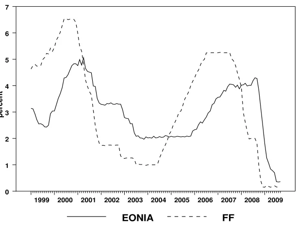
Figure 1 displays the U.S. Federal Funds Rate – the overnight interest rate closely

con-trolled by the Federal Reserve – and its counterpart in the Euro area the EONIA. Both

time series are monthly averages of daily data. The ﬁgure suggests that monetary

pol-icy in the Euro area follows that of the U.S. with a lag. The cross correlation coeﬃcient

peaks at a lag of seven months for the Federal Funds Rate. This relationship between

policy interest rates in the Euro area and the U.S. has been studied empirically by Belke

and Gros (2003, 2005, 2006). They investigate the dynamic interrelationship between

Euro area and U.S. short-term interest rates using Granger causality tests with daily

and weekly observations. For the time period before September 2001 they ﬁnd a

sym-metric relationship with either bi-directional Granger causality or no Granger causality

at all depending on the chosen lag length. Using observations from after September

2001 only, they present evidence for an asymmetric relationship with Granger causality

running from the Federal Funds Rate to the Euro area interest rate. The analysis of

the short-run interest-rate interactions between the Euro and the U.S. is extended in

Belke and Cui (2010) to simultaneously account for a possible long-run relationship.

Using a vector-error-correction model (VECM) and monthly data they estimate a

(4)

EONIA FF

percent

1999 2000 2001 2002 2003 2004 2005 2006 2007 2008 2009 0

[image:4.612.128.433.82.321.2]

1 2 3 4 5 6 7

Figure 1: EONIA and Federal Funds Rate

the existence of a long-run equilibrium relation between both interest rates. For the

short-run interest-rate dynamics their estimates indicate for both interest rates similar

speeds of adjustment to deviations from this long-run equilibrium.

One possible explanation for the lead-lag pattern in Figure 1 is that both central banks

change their interest rates according to movements in the business cycle and that the

Euro area business cycle lags that of the U.S. (e.g. Begg et al., 2002). This eﬀect can be

accounted for by estimating interest rate reaction functions for the central banks that

include macroeconomic variables and control for the stage of the business cycle. Breuss

(2002) and Ullrich (2005) estimate Taylor rules for the ECB augmented by the lagged

Federal Funds Rate and show that the U.S. interest rate enters the Euro area

mone-tary policy reaction function in a statistically signiﬁcant way. Belke and Cui (2010)

augment their VECM by Euro area and U.S. inﬂation rates and output gaps. Their

results still indicate a cointegrating relationship between the EONIA and the Federal

Funds Rate. However, the U.S. interest rate is estimated to be weakly exogenous to

the VECM indicating an asymmetry in the relationship between the ECB and the Fed

by which only the ECB and not the Fed responds to deviations from the

cointegrat-ing relation. Scotti (2006) analyses the interdependence of the timcointegrat-ing of interest-rate

changes by the ECB and the Fed and controls for the eﬀects of output and inﬂation

(5)

on the interest-rate decisions. She estimates a bivariate conditional hazard model on

weekly data and ﬁnds evidence for contemporaneous interdependence in the timing of

interest rates changes by the two central banks.

The patterns found empirically in the time-series of policy interest rates are the result

of the monetary policy reaction functions of the Fed and the ECB. These reaction

functions link the setting of the short-term interest rate by the central banks to other

macroeconomic variables. Correlation between the interest rates set by both central

banks can be caused by one or both central banks reacting directly to the

interest-rate chosen by the other one or by both central banks reacting to the same or similar

macroeconomic variables, perhaps with diﬀerent time lags and intensities. Theoretical

analyses of monetary policy reaction functions (e.g. Clarida et al., 1999; Galí, 2008;

Svensson, 1997; Woodford, 2003a) show that an optimal reaction function makes the

central bank respond to all variables and shocks that help in forecasting the central

bank’s goal variables. This implies, that it will be optimal for the ECB to react to

U.S. macroeconomic variables if these have predictive power for Euro area inﬂation

and economic activity, either because these variables directly or indirectly aﬀect the

Euro area economy or because they convey information about shocks that are relevant

to the Euro area.

In this paper, we study how far this explanation takes us in reproducing the observed

correlations of short-term interest rates in the U.S. and the Euro area. From an

em-pirically estimated VAR model of the U.S. and Euro area we construct an optimal

monetary policy reaction function for the ECB and investigate how important the

op-timal responses to U.S. variables and shocks are in determining the time path of the

EONIA. By means of simulations we show that the optimal reaction function can

re-produce the observed interest-rate correlation pattern to a large extent and that its

reactions to the various shocks in the model are close to those for the reaction function

estimated on the observed data. Our results suggest that the observed interest-rate

correlation between the U.S. and the Euro area results from the optimal reaction of

the ECB to U.S. variables and U.S. shocks.

The main results of the paper are as follows: (1) It is shown that the observed monetary

policy function of the ECB can be approximated by an optimal reaction function

(6)

policy implies strong reactions to shocks to U.S. variables, particularly to the Federal

Funds Rate and induces a high correlation between the interest rates set by the ECB

and the Fed. (3) These results are robust with respect to changes in the identiﬁcation

assumptions of the VAR and to the introduction of uncertainty about the monetary

transmission mechanism.

The next section derives an optimal monetary policy reaction function for the ECB

from an estimated structural VAR (Section 2.1) and presents results for the importance

of U.S. variables in the optimal reaction function and for its ability in reproducing the

observed time series of the EONIA and its correlation with the Federal Funds Rate

(Section 2.2). Section 3 investigates the robustness of these results by considering

alternative identiﬁcation schemes for the structural VAR. Section 4 presents results

for a model which introduces uncertainty about the structural relationships in the

economy. The results from the accordingly adjusted optimal monetary policy reaction

function resemble closely those from Section 2. Section 5 summarizes the results and

concludes.

2 Optimal policy with additive uncertainty

We construct the optimal monetary policy reaction function for the ECB from an

esti-mated structural VAR model of the Euro area and the U.S. economies using a

method-ology proposed in Sack (2000). The VAR framework is a natural way to model the

implications of macroeconomic interdependence on the monetary policy of both central

banks. A VAR that includes both policy interest rates together with macroeconomic

variables that are important determinants of monetary policy such as unemployment,

output and inﬂation is a ﬂexible and relatively unrestricted framework that can account

for both the systematic responses of the central banks to the macroeconomy and for

the macroeconomic interdependence of the U.S. and the Euro area. It allows to

esti-mate the monetary policy reaction functions of the ECB and the Fed and to study the

central banks’ reaction functions by means of impulse response analyses and variance

decompositions. Furthermore, VAR models have already been successfully applied to

studies of monetary policy interdependence, although mostly for small open economies.

(7)

The interrelation between the U.S. Federal Funds Rate and interest rates in other

countries has been studied with structural vector autoregressions by Grilli and Roubini

(1995). They estimate structural VARs for non-U.S. G-7 countries either individually

or as a group and add an indicator of U.S. monetary policy to this model. They show

that unexpected innovations in the Federal Funds Rate lead to signiﬁcant changes in

the short-term interest rates of non-U.S. G-7 countries. The transmission channels of

U.S. monetary policy shocks to the other G-7 countries are studied in more detail by

Kim (2001) using a sample period from 1974 to 1996. He augments a VAR model for

the U.S. with individual variables for the other G-7 countries. Although output and

production in the other countries increase signiﬁcantly after an expansionary monetary

policy shock in the U.S. he ﬁnds these shocks to have little eﬀect on the other countries’

trade balances and short-term interest rates. He concludes that expansionary monetary

policy impulses are transmitted from the U.S. to the other economies via their eﬀects

on world interest rates. Neri and Nobili (2010) build structural VAR models of the

Euro area and the U.S. combined to study the eﬀects of U.S. monetary policy shocks

on the Euro area. They estimate a signiﬁcantly positive response of the Euro area

short-term nominal interest rate to an exogenous increase in the Federal Funds Rate.

Other authors have not focussed explicitly on the eﬀects of U.S. monetary policy shocks

on other countries’ interest rates. Nevertheless, they have incorporated in their VAR

models the assumption of a dependence of the country of interest’s monetary policy

on the U.S. For example, Cushman and Zha (1997) study the eﬀects of monetary

policy shocks on the Canadian economy and account explicitly for the dependence

of Canadian monetary policy on the U.S. Federal Funds Rate. Kim and Roubini

(2000) investigate the eﬀects of monetary policy shocks on exchange rates for small

open economies and use the Federal Funds Rate to control for the eﬀects of foreign

monetary policy. Brischetto and Voss (1999) adapt the structural VAR model of Kim

and Roubini (2000) to estimate the eﬀects of monetary policy shocks on the Australian

economy and, again, include the Federal Funds Rate as an indicator of foreign monetary

policy.

This VAR literature does, however, only shed limited light on the question of

interest-rate correlation. Its focus is mostly on the unsystematic part of monetary policy, i.e.

(8)

is driven by the systematic reactions of monetary policy to the whole range of shocks.

Hence, in this paper we will focus on how monetary policy responds to a variety

of shocks as opposed to how the other variables respond to monetary policy shocks.

Furthermore, our approach enables us to consider optimal interest rate reactions and

to use these to evaluate the actually observed behavior of the central banks.

2.1 The optimal monetary policy reaction function of the ECB

The starting point of the analysis is an estimated structural vector autoregression

(VAR)

Zt = kZ+ q

i=0

A_i_Z_t−_i+

q

i=0

b_i_R_t−_i+ℓ_Zt+ν

Z

t (1)

Rt = kR+ q

i=0

c′

iZt−i+ q

i=1

diRt−i+ℓRt+νtR. (2)

Zt is an (n×1)-vector of non-policy variables, Rt is the ECB policy interest rate, q is

the number of lags in the VAR,νZ

t is a(n×1)-vector of uncorrelated structural shocks

that is also uncorrelated with the structural policy disturbance νR

t . kZ is a vector

of constants, ℓZ a vector of coeﬃcients on time trends and kR and ℓR the constant

and time trend in the estimated monetary policy reaction function. A_i _are ₍_n ×n)

coeﬃcient matrices and b_i _and c_i _are ₍_n _× ₁₎ _{coeﬃcient vectors.} A₀ _{describes the}

contemporaneous interactions of the non-policy variables whileb₀ _{gives the immediate}

(if any) reactions of the variables in Zt to the monetary policy instrument Rt.

Non-zero elements in c₀ _{indicate to which of the variables in} _Z_t _{monetary policy responds}

to within the same period.

In this paper’s application the variables in Zt are the deviations of the U.S. and Euro

area unemployment rates from their natural levels (U N U S, U N EM U), the growth

rates of industrial production in the U.S. and in the Euro Area (IP U S,IP EM U), rates

of consumer price inﬂation in the U.S. and in the Euro Area (IN F LU S,IN F LEM U),

a smoothed rate of commodity price inﬂation P COM, the Federal Funds Rate (F F)

and the nominal U.S.-Dollar/Euro exchange rate (EXCHR). The monetary policy

indicatorRt is approximated by the EONIA rate, the average overnight interest rate in

the Euro area interbank market. As shown in (1) the VAR includes constants and time

(9)

trends. The speciﬁcation in inﬂation rates and growth rates is chosen in accordance

with the variables included in the central bank’s loss function below.1

Equation (2) represents a backward-looking monetary policy reaction function (MPRF)

of the ECB. Its estimate can be obtained from the estimated structural VAR that

results from stacking the non-policy variablesZtand the monetary policy indicatorRt.

Equations (1) of the structural VAR can be rewritten in state-space form as a transition

equation for the state vectorXt

Xt+1 =FXt+HRt+J+µt+1, (3)

where the coeﬃcients inF_,H_,J _{can be derived from the coeﬃcients in (1). The state}

vector Xt contains current and lagged values of the variables in Zt and lags of the

EONIA. The immediate eﬀects of monetary policy on the state variables are captured

by the vector H_.

The state-space representation of the structural model of the economy (3) can be used

to derive an optimal monetary policy reaction function (e.g. Mandler, 2009; Sack,

2000): The ECB is assumed to maximize a quadratic objective function

−1

2Et

∞

i=1 βi

(πt+i−π

∗

)2+λu(ut+i−u

∗

)2+λR(Rt+i−1−Rt+i−2)

2

. (4)

This is a standard objective function used in monetary policy analysis that penalizes

the central bank for deviations of unemployment and inﬂation from their target values

u∗

and π∗

(e.g. Walsh, 2010). The presence of the squared change in the interest

rate Rt+i−₁ − R_t₊_i−₂ represents an aversion to interest rates changes and leads to

interest-rate smoothing by the central bank (e.g. Woodford, 2003b).2

λu and λR are

the weights attached to the employment and interest-rate objectives relative to the

inﬂation objective and β is a discount factor. Since the unemployment variables inZt

are already deﬁned as deviations of unemployment rates from their natural levels, u∗

is equal to zero, i.e. the ECB is assumed to target the natural rate of unemployment.

The part of the objective function in square brackets can be written in a notation

1

Detailed information on the data is given in the appendix.

2

Empirically, interest rate smoothing manifests in a statistically signiﬁcant and quantitatively

(10)

compatible with (3)

(Xt+i −X

∗

)′

G₍_X_t₊_i−X∗

). (5)

G _{has as non-zero entries only the elements corresponding to the weights attached to}

the relevant variables inXt+i in the objective function. X∗ is the vector of target values

for the state variables. In this model the only non-zero element in X∗

corresponds to

the inﬂation target π∗

. 3

The optimal policy reaction function determines the policy instrumentRtas a function

of the state variables Xt and maximizes (4) subject to (3). This linear-quadratic

dynamic programming problem can be solved using standard methods (e.g. Ljunquist

and Sargent, 2004, Ch. 4; Sack, 2000). The optimal monetary policy reaction function

solves the Bellman equation

V(Xt) = max Rt

−(Xt−X

∗

)′

G₍_X_t−X∗

) +βEt[V(Xt+1)]

, (6)

subject to (3). For a linear quadratic dynamic programming problem like this the value

function has the form

V(X) =X′

tΛXt+ 2X

′

tω+ρ, (7)

with constants Λ,ω and ρ. The solution for the optimal policy reaction function is

R∗

t =−(H

′_ΛH

)−1

(H′_ΛF

Xt+H

′_ΛJ

+H′

ω), (8)

where the symmetric matrixΛ _{is deﬁned implicitly by the Riccati equation}

Λ₌−G₊_βF′

ΛF−βF′

ΛH₍H′

ΛH₎−1H′

ΛF_. ₍₉₎

The vector ω is given by

ω = I−βF′

I−ΛH₍H′

ΛH₎−1H

−1

× G_X∗

+βF′

Λ I−H₍H′

ΛH₎−1H′

ΛJ_. ₍₁₀₎

3

A slight departure from the standard speciﬁcation is the use ofRt+i₋1−Rt+i₋2instead ofRt+i−

Rt+i₋1 in (4). Through this modiﬁcation, the objective function can be written in terms of the state

variables as given in (5). The difference of (4) to the standard specification caused by this modification

is twofold: First, in the inﬁnite sum in equation (4) the term Rt+i−Rt+i₋1 is multiplied by β

i+1

instead ofβi

as in the standard formulation and, second, the objective function (4) includes the term

−(1/2)β(Rt₋1−Rt₋2)which would not be present when using the standard speciﬁcation. β is close to one andRt₋1−Rt₋2 does not depend on the setting of the interest rate in periodt. Hence, these

two diﬀerences will have a negligible eﬀect on the optimal monetary policy reaction function.

(11)

Under the optimal monetary policy reaction function the dynamics of the economy are

given by (3) and (8). (8) shows how the value of the monetary policy instrumentRt is

determined by the current state of the economy Xt. Xt and Rt in turn determine the

state vector in the next period Xt+1 according to (3). The only sources of uncertainty

are the shocks µt+1 to the transition equation (3). The optimal monetary policy

reac-tion funcreac-tion (8) is much less restrictive than a Taylor-type rule and allows the policy

rate to react to current and lagged values of all of the non-policy variables and to lags

of the policy interest rate.

In deriving the optimal ECB reaction function (8) we treat (3) as a structural

represen-tation of the economy, i.e. we assume the coeﬃcients in (3) that are derived from the

estimated structural VAR to be invariant with respect to changes in the ECB reaction

function. This assumption can be questioned in the light of the Lucas (1976) critique.

Since the parameters in lagged representations of an economic model as in (1) and (2)

depend on agents’ expectations of monetary policy they will change when the central

bank is assumed to follow a monetary policy diﬀerent from that in the estimation

pe-riod.

However, the empirical relevance of the critique depends on the size and on the

eco-nomic signiﬁcance of the changes in the reduced form parameters that are caused by

alternative policies. For example, even though much evidence has been presented for

pronounced changes in the Fed’s monetary policy reaction function, empirical VAR and

backward-looking non-VAR models appear to be stable, see, for example Rudebusch

and Svensson (1999), Bernanke and Mihov (1998), and Estrella and Fuhrer (2003).4

Rudebusch (2005) conducts a thorough investigation into the empirical relevance of

the Lucas critique. He simulates structural economic models that contain

expecta-tional variables and ﬁnds only very modest changes in the reduced form coeﬃcients.

In most cases, he is unable to reject the null hypothesis of stability in the reduced

form parameters after having changed the policy rule. That structural invariance in

face of plausible policy changes often cannot be rejected is argued as well by Estrella

and Fuhrer (2003). In the following section we will show that the optimal monetary

policy reaction function is actually a good approximation to the actual one and that

4

In the context of estimated Taylor rules see, for example, Boivin (2006), Clarida, Galí, and Gertler

(12)

the behavior of the economy model under the optimal ECB reaction function is close

to that of the estimated VAR. Hence, the possible eﬀect of the Lucas critique will be

very limited.

The ﬁrst step in the construction of the optimal monetary policy reaction function for

the ECB is the estimation of the structural VAR (1) and (2) and its transformation into

the state space model (3). Structural identiﬁcation of the VAR is achieved by imposing

zero restrictions in the matrix A₀ _{of contemporaneous interactions of the non-policy}

variables in (1), in the vectorb₀ _{in (1) indicating the immediate reactions of the}

non-policy variables to the monetary non-policy instrument, and in the vector c₀ _{in (2) which}

represents the within-period response of monetary policy to the non-policy variables.

Of special importance are the restrictions imposed on c₀ _{since these restrict to which}

non-policy variables monetary policy can respond immediately, i.e. of which non-policy

variables the current observations are in the central bank’s information set. This has

implications for the construction of the state vector Xt in (3) since comparisons of

the optimal and the estimated monetary policy reaction functions must be based on

identical information sets: The current observations of all of the variables with non-zero

elements in c₀ _{must be included in} _X_t_.

In our model the identiﬁcation of the structural VAR is based on the following

as-sumptions:5

For both the EMU and the U.S. variables we assume recursive orderings

in which the unemployment rate is ordered ﬁrst, followed by the growth rate of

indus-trial production and by the inﬂation rate. There is no contemporaneous interaction

of these variables across country blocks which is a reasonable assumption for monthly

data. As in Kim and Roubini (2000) we include an indicator of commodity price

infla-tion to capture global inflainfla-tionary shocks. Commodity price inflainfla-tion reacts to all other

variables with a lag. The nominal exchange rate is aﬀected within the same period by

all other variables including the interest rates in the Euro Area and in the U.S.

Of particular importance are the identiﬁcation assumptions concerning monetary

pol-icy in the U.S. and in the Euro Area. In the ﬁrst version of the model we assume

5

These identifying assumptions are in part derived from the standard standard recursive

identiﬁ-cation scheme common in the literature (e.g. Christiano et al., 1999). This structure for variables

within one economy is also used in Kim (2001).

(13)

that U.S. monetary policy reacts within the same period to unemployment, industrial

production and inﬂation in both regions and to commodity price inﬂation but not to

the ECB’s monetary policy and to the exchange rate. The ECB is assumed to react

within the same period to all variables except for the exchange rate, i.e. the ECB is

allowed to respond immediately to U.S. monetary policy. Since this implies an

asym-metry in the treatment of both central banks we will also present results in Section 3

for slightly diﬀerent identiﬁcation schemes and show that our results are robust with

respect to these changes. In particular, we also consider a model in which the ECB

does not react to U.S. monetary policy within the current period while the Federal

Reserve immediately reacts to changes in Euro area interest rates.6

The structural VAR is estimated on monthly data from 1995:7 to 2007:12.7

Since a

VAR with ten variables is ﬁtted to a relatively short sample period the VAR is

esti-mated with only six lags.

2.2 Results

The optimal monetary policy reaction function (8) contains four free parameters: the

discount factor β, the relative weights of unemployment and interest-volatility in the

central bank’s objective function,λu andλR, and the inﬂation targetπ∗. As suggested

by Sack (2000) we impose β = 0.996 and estimate λu, λR and π

∗

by minimizing the

sum of squared deviations of the interest rate implied by (8) from the actually observed

interest rate.8

For any combination ofλu,λRandπ

∗

on a grid we compute the optimal

monetary policy reaction function (8) and use it to obtain a time series of optimal

interest rates based on the historically observed values for the state variables in Xt.

The particular combination of λu, λR and π∗ selected is the one which minimizes the

sum of squared deviations of the optimal from the observed EONIA rate for 1999M1

6

Kim (2001) considers various structural and recursive identiﬁcation schemes in his VAR study on

the international transmission of monetary policy shocks and shows his results to be very robust with

respect to these changes.

7

Including observations up to the collapse of Lehman Brothers in September 2008 resulted in a

large increase in the imprecision of the estimates indicating the possibility of a structural break.

8

The estimation of structural parameters in an optimal monetary policy rule by ﬁtting it to observed

(14)

EONIA EONIA(opt)

percent

1999 2000 2001 2002 2003 2004 2005 2006 2007 0

[image:14.612.127.431.82.321.2]

1 2 3 4 5 6

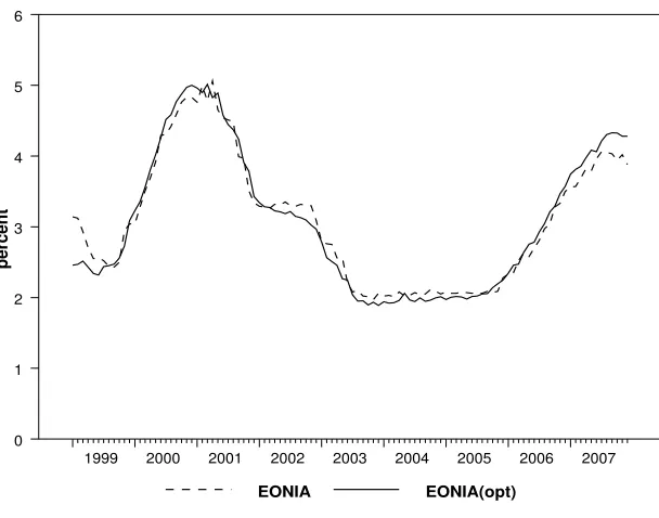
Figure 2: Actual and ﬁtted optimal EONIA

to 2007M12.9

The results of this search procedure showed a tendency for λR to

be-come excessively large while the estimates for the other two parameters were mostly

independent of λR. Hence, we ﬁxed λR = 2.5 at a value which provided a reasonably

good approximation to the observed time series of the EONIA and searched over λu

andπ∗

only. Higher values forλR led to only very small improvements in the ﬁt of the

model. The resulting estimate for the weight on unemployment isλu = 0.0575and the

estimate for the inﬂation target is π∗

= 2.20 percent which is only slightly above the ECB’s oﬃcial inﬂation target of two percent. The estimated weight on the

unemploy-ment objective is relatively low but in line with other results in the literature. Using

quarterly data for the period 1980:3-1998:3 Favero and Rovelli (2003) ﬁnd a weight of

0.00125 on the output gap in the loss function of the Federal Reserve. Also for the

Federal Reserve, Dennis (2001, 2004) reports statistically insigniﬁcant estimates of the

weight on the output gap while Collins and Siklos (2004) estimate a weight of 0.001.

Figure 2 shows the observed time series for the EONIA together with the one

con-structed from the optimal monetary policy reaction function. Except for the ﬁrst and

last few months the optimal interest rate path tracks the observed one very closely

9

Since no explicit solution for the matrixΛ_{in (9) exists this search procedure is employed. As a}

consequence information on the precision of the estimates is not available.

(15)

EONIA(opt)_t,FF_t-i EONIA_t,FF_t-i

lag for FF (months)

correlation coefficient

-26 -22 -18 -14 -10 -6 -2 2 6 10 14 18 22 26 -0.6

[image:15.612.124.437.84.317.2]

-0.4 -0.2 0.0 0.2 0.4 0.6 0.8 1.0

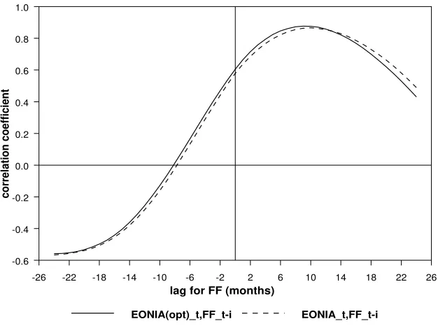
Figure 3: Correlation of actual and ﬁtted optimal EONIA with observed

Fed-eral Funds Rate

with a sum of squared deviations of 3.50. The volatility of the optimal interest rate is

slightly above the volatility of the observed EONIA (standard deviations of 0.98 and

0.90, respectively). The optimal monetary policy reaction function is able to reproduce

the cross correlation structure of the EONIA and the observed Federal Funds Rate at

leads and lags up to two years as presented in Figure 3.

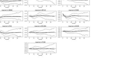
Figure 4 compares impulse responses of the EONIA for the estimated monetary policy

reaction function to those for the optimal one. The impulse responses for the optimal

monetary policy reaction functions (MPRF) (solid lines) are obtained from simulating

the structural equations for the non-policy variables in (3) together with the optimal

monetary policy reaction function (8). The identiﬁcation assumption concerning the

ECB’s information set used to compute the optimal reaction function is identical to the

one imposed in the estimation of the structural VAR. Therefore, the impulse responses

for the system with the optimal reaction function are simulated with the same

struc-tural shocks as used for the estimated impulse responses.10

For the structural shocks

10

This assumes the estimated structural shocks from the VAR as the ’true’ shock series and simulates

the eﬀects on the dynamical adjustment of the economy of exchanging the estimated for the optimal

(16)

impulse responses for EONIA: with optimal MPRF (solid), with estimated MPRF (dashed)

response to UNUS

months

0 10 20 30 40 50 -0.10 -0.05 0.00 0.05 0.10 0.15

response to UNEMU

months

0 10 20 30 40 50 -0.15 -0.10 -0.05 0.00 0.05 0.10 0.15 0.20

response to IPUS

months

0 10 20 30 40 50 -0.15 -0.10 -0.05 0.00 0.05 0.10 0.15 0.20

response to IPEMU

months

0 10 20 30 40 50 -0.25

-0.15 -0.05 0.05 0.15

response to INFLUS

months

0 10 20 30 40 50 -0.20

-0.10 -0.00 0.10 0.20

response to INFLEMU

months

0 10 20 30 40 50 -0.20

-0.10 -0.00 0.10 0.20

response to PCOM

months

0 10 20 30 40 50 -0.15 -0.10 -0.05 0.00 0.05 0.10 0.15 0.20

response to FF

months

0 10 20 30 40 50 -0.15 -0.10 -0.05 0.00 0.05 0.10 0.15

response to EONIA

months

0 10 20 30 40 50 -0.15 -0.10 -0.05 0.00 0.05 0.10 0.15

response to EXCHR

months

[image:16.612.155.726.111.467.2]

(17)

to the EONIA itself we use the estimate from the policy equation in the structural

VAR (2). The dashed lines are the impulse responses for the EONIA in the estimated

structural VAR ((1) and (2)) and the dotted lines represent 90% probability bands

around the estimated impulse responses and were constructed by Monte Carlo

simu-lation.11

For many of the shocks the impulse responses of the model with the optimal

reaction function imposed are close to the estimated impulse responses and follow very

similar trajectories. The optimal impulse responses match the estimated ones very

suc-cessfully in the ﬁrst year after shocks to the EMU unemployment rate, U.S. industrial

production and to the EONIA itself. The optimal reaction function leads to a quicker

but shortly lived negative (positive) interest rate response to shocks to U.S. (EMU)

inﬂation compared to the estimated reaction of the EONIA. The response of the

EO-NIA to Federal Funds Rate shocks within the ﬁrst few months is more pronounced for

the optimal reaction function but less persistent. Both the optimal reaction function

and the estimated one imply a hump-shaped response to Federal Funds Rate shocks

similar to the result in Neri and Nobili (2010). Strong changes can be observed for

the response to U.S. unemployment, Euro area industrial production and to

commod-ity price inﬂation. Overall, the impulse responses from the optimal monetary policy

reaction function provide a reasonably good approximation to the estimated responses

of the ECB. Figures 5 and 6 oﬀer the same comparisons for the impulse responses of

the EMU unemployment and inﬂation rates. Again, the impulse responses from the

VAR with the optimal monetary policy reaction function imposed are very close to the

estimated ones.

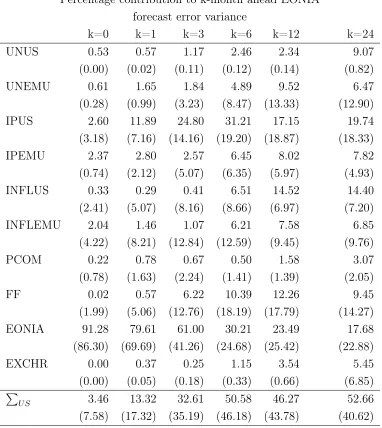
Table 1 presents decompositions of the EONIA forecast variance for the model with,

ﬁrst, the estimated and then the optimal ECB reaction functions imposed. Again,

because of the identical identiﬁcation assumptions we use the VAR estimates of the

structural shocks to construct the variance decompositions for the system including

the optimal reaction function.

A few interesting facts emerge: The contribution of inﬂation shocks both in the U.S.

and in the EMU is higher under the optimal ECB reaction function than that under

11

The dynamical stability of the model obtained from combining (3) and (8) was checked by

com-puting the largest absolute eigenvalue of the system as 0.996. The largest absolute eigenvalue of the

(18)

impulse responses for INFLEMU: with optimal MPRF (solid), with estimated MPRF (dashed)

months

0 10 20 30 40 50 -0.15 -0.10 -0.05 0.00 0.05 0.10 0.15

months

0 10 20 30 40 50 -0.15 -0.10 -0.05 0.00 0.05 0.10 0.15 0.20

months

0 10 20 30 40 50 -0.15 -0.10 -0.05 0.00 0.05 0.10 0.15

months

0 10 20 30 40 50 -0.20 -0.15 -0.10 -0.05 -0.00 0.05 0.10 0.15

months

0 10 20 30 40 50 -0.20

-0.10 -0.00 0.10 0.20

months

0 10 20 30 40 50 -0.20

-0.10 -0.00 0.10 0.20

months

0 10 20 30 40 50 -0.20 -0.15 -0.10 -0.05 -0.00 0.05 0.10 0.15

response to FF

months

0 10 20 30 40 50 -0.15 -0.10 -0.05 0.00 0.05 0.10 0.15

months

0 10 20 30 40 50 -0.15 -0.10 -0.05 0.00 0.05 0.10 0.15

months

[image:18.612.147.721.110.468.2]

(19)

impulse responses for UNEMU: with optimal MPRF (solid), with estimated MPRF (dashed)

months

0 10 20 30 40 50 -0.050

-0.025 0.000 0.025 0.050

months

0 10 20 30 40 50 -0.06 -0.04 -0.02 0.00 0.02 0.04 0.06

months

0 10 20 30 40 50 -0.050 -0.025 0.000 0.025 0.050 0.075

months

0 10 20 30 40 50 -0.04 -0.02 0.00 0.02 0.04 0.06 0.08

months

0 10 20 30 40 50 -0.08 -0.06 -0.04 -0.02 0.00 0.02 0.04 0.06

months

0 10 20 30 40 50 -0.050 -0.025 0.000 0.025 0.050 0.075 0.100 0.125

months

0 10 20 30 40 50 -0.100 -0.075 -0.050 -0.025 -0.000 0.025 0.050

response to FF

months

0 10 20 30 40 50 -0.04 -0.02 0.00 0.02 0.04 0.06

months

0 10 20 30 40 50 -0.05

-0.03 -0.01 0.01 0.03

months

[image:19.612.153.718.109.469.2]

(20)

[image:20.612.95.477.224.652.2]

Table 1: Comparison of variance decompositions under estimated and

opti-mal MPRF

Percentage contribution to k-month ahead EONIA forecast error variance

k=0 k=1 k=3 k=6 k=12 k=24

UNUS 0.53 0.57 1.17 2.46 2.34 9.07

(0.00) (0.02) (0.11) (0.12) (0.14) (0.82)

UNEMU 0.61 1.65 1.84 4.89 9.52 6.47

(0.28) (0.99) (3.23) (8.47) (13.33) (12.90)

IPUS 2.60 11.89 24.80 31.21 17.15 19.74

(3.18) (7.16) (14.16) (19.20) (18.87) (18.33)

IPEMU 2.37 2.80 2.57 6.45 8.02 7.82

(0.74) (2.12) (5.07) (6.35) (5.97) (4.93)

INFLUS 0.33 0.29 0.41 6.51 14.52 14.40

(2.41) (5.07) (8.16) (8.66) (6.97) (7.20)

INFLEMU 2.04 1.46 1.07 6.21 7.58 6.85

(4.22) (8.21) (12.84) (12.59) (9.45) (9.76)

PCOM 0.22 0.78 0.67 0.50 1.58 3.07

(0.78) (1.63) (2.24) (1.41) (1.39) (2.05)

FF 0.02 0.57 6.22 10.39 12.26 9.45

(1.99) (5.06) (12.76) (18.19) (17.79) (14.27)

EONIA 91.28 79.61 61.00 30.21 23.49 17.68

(86.30) (69.69) (41.26) (24.68) (25.42) (22.88)

EXCHR 0.00 0.37 0.25 1.15 3.54 5.45

(0.00) (0.05) (0.18) (0.33) (0.66) (6.85)

U S 3.46 13.32 32.61 50.58 46.27 52.66

(7.58) (17.32) (35.19) (46.18) (43.78) (40.62)

NOTES: Sample period is 1995:7-2007:12. Numbers in brackets apply to the model including the optimal MPRF, number without brackets to the estimated VAR.

(21)

Actual and simulated optimal EONIA - historical shocks

EONIA(opt) EONIA

percent

1999 2000 2001 2002 2003 2004 2005 2006 2007 0

1 2 3 4 5 6

Actual and simulated Federal Funds Rate - historical shocks

FF(sim) FF

percent

1999 2000 2001 2002 2003 2004 2005 2006 2007 0

[image:21.612.126.439.96.308.2]

1 2 3 4 5 6 7 8

Figure 7: Simulation of EONIA and Federal Funds Rate with historical

shocks

the estimated one for forecast horizons up to six months. The importance of shocks to

industrial production in explaining unexpected EONIA changes declines. U.S.

unem-ployment shocks explain less variation in the EONIA under the optimal ECB reaction

function than under the estimated one while the explanatory power of EMU

unem-ployment shocks increases for forecast horizons of three months and more. In addition,

the contribution of Federal Funds Rate innovations to the EONIA forecast variance

in-creases strongly while that of the EONIA’s own shocks declines in the short run. The

last two rows show the aggregate variance contribution of all U.S. variables together.

For forecast horizons up to three months the optimal monetary policy reaction

func-tion recommends assigning a greater importance to U.S. shocks than actually observed.

After three months the aggregate contribution of U.S. shocks to the EONIA is similar

for the optimal and for the estimated reaction function.

The time series for the optimal EONIA in Figure 1 was derived by computing the

optimal EONIA rate for the actually observed values of the state variables in Xt at

(22)

EONIA(opt)_t,FF(sim)_t-i EONIA_t,FF_t-i

-26 -22 -18 -14 -10 -6 -2 2 6 10 14 18 22 26 -0.6

[image:22.612.124.437.83.317.2]

-0.4 -0.2 0.0 0.2 0.4 0.6 0.8 1.0

Figure 8: Correlation of simulated EONIA and simulated Federal Funds Rate

that result from simulating (3) with the optimal monetary policy reaction function (8).

For each model the historical time series of the structural shocks were constructed from

the reduced form VAR residuals using the identiﬁcation assumptions given in Section

2.1. Beginning at the historically observed values for the state vector Xt in 1999:1

each model is simulated subject to the estimated time series of structural shocks. This

assumes all variables in the model to evolve according to their dynamics in (3) and (8)

and does not reset them to their observed values in each period. In Figure 7 the model

is still able to capture broadly the evolution of the policy interest rates in the U.S. and

in the EMU.12

Figure 8 displays the correlation coeﬃcients between the simulated EONIA and Federal

Funds Rates series in Figure 7 at various leads and lags and shows the correlation

patterns to be very close to those of the observed time series for leads and lags of the

Federal Funds Rate of up to about a year. However, the model has some problems in

replicating the long-run correlations between the two interest rate series which are too

weak compared to the observed ones.

12

Note that only for the ECB an optimal monetary policy reaction function is used. For the Fed

the model still includes the estimated reaction function.

(23)

All these results indicate that shocks to U.S. macroeconomic variables are important

driving forces behind the dynamic behavior of the EONIA even though the U.S.

vari-ables enter the optimal monetary policy reaction function only because of their

pre-dictive power for inﬂation and unemployment in the Euro area. In fact, the optimal

monetary policy reaction assigns an even greater importance to short-run reactions

to U.S. variables than estimated. Compared to the estimated ECB reaction function

the optimal one implies a stronger reaction to unexpected Federal Funds Rate changes

within the ﬁrst months and emphasizes the importance of U.S. monetary policy shocks

for the EONIA. The correlation pattern between the EONIA and the Federal Funds

Rate is thus caused by the direct response of each central bank to the other’s policy

interest rate and by the two central banks reacting to changes in the macroeconomic

variables in both the U.S. and the Euro area. In the context of the model presented in

this paper, this behavior of the ECB is close to optimal.

3 Robustness

The results in the preceding model were derived from a structural VAR in which the

Federal Reserve reacts to U.S. and Euro area unemployment, industrial production and

inﬂation and to commodity price inﬂation within a given month. The Federal Reserve

was assumed to respond to the EONIA with a lag of month. In contrast, the ECB was

allowed to react immediately to unemployment, industrial production and inﬂation in

both the Euro area and the U.S. and to commodity price inﬂation as well as to the

Federal Funds Rate. This identiﬁcation assumption was important in deriving the

state equation for the economy (3) and the structural shocks used to construct impulse

responses, variance decompositions and the simulated interest rate series in Figure 7.

In order to investigate how strongly our results depend on this assumption we derived

results as in Section 2 for different identification schemes. The difference in model 1 to

the benchmark model in Section 2 is that it restricts the set of variables the Federal

Reserve is assumed to react to within the month to only U.S. unemployment, industrial

production and inﬂation and to commodity price inﬂation. It retains the assumption

(24)

[image:24.612.110.461.106.177.2]

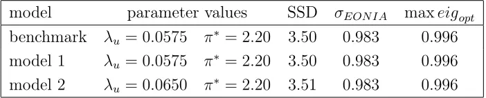
Table 2: Estimation results for various identiﬁcation schemes

model parameter values SSD σEON IA maxeigopt

benchmark λu = 0.0575 π

∗

= 2.20 3.50 0.983 0.996

model 1 λu = 0.0575 π

∗

= 2.20 3.50 0.983 0.996

model 2 λu = 0.0650 π

∗

= 2.20 3.51 0.983 0.996

SSD: Sum of squared deviations of optimal from observed EONIA.

σEON IA: Standard deviation of fitted EONIA (standard deviation of

observed EONIA is 0.900). maxeig_opt is the largest absolute Eigen-value of the model with the optimal MPRF imposed. The largest absolute eigenvalue of the estimated VAR is 0.998.

Model 2 switches the information assumptions of the benchmark model between the

Federal Reserve and the ECB around and assumes that the Federal Reserve reacts

immediately to U.S. and Euro area unemployment, industrial production and inﬂation

and to commodity price inﬂation as well as to the EONIA while the ECB does not

react to the Federal Funds Rate within the month.13

The estimates for the parameters in the central bank’s loss function (4) are almost

the same across models.14

The ﬁt of the optimally set EONIA to the observed one is

almost identical for for the benchmark model and models 1 and 2 as shown in Figure

9. For all models, the correlation between the ﬁtted EONIA and the Federal Funds

Rate comes close to the one of the observed EONIA (Figure 10).

Figure 11 presents for all models the impulse responses of the EONIA if each optimal

monetary policy reaction function is combined with the appropriate version of the

state equation (3) for the model. The structural shocks used in this simulation are

that from the structural VAR with identiﬁcation assumptions consistent with those

used to construct the optimal monetary policy reaction function. The dashed lines

13

We estimated also a third model which assumed that both central banks react to each other’s

in-terest rate changes immediately but to ensure identiﬁcation, restricted the Federal Reserve to respond

to the other Euro area variables except for the EONIA with a lag of one month. Unfortunately, there

were diﬃculties in estimating the contemporaneous interaction coeﬃcients inA0, b0 and c0 between

the variables not only for this speciﬁcation but also for slightly diﬀerent models with the assumption

of immediate interaction between the ECB and the Fed. Furthermore the impulse responses indicated

that the interest rate shocks were not identiﬁed appropriately. These problems could be avoided by

replacing the U.S.-Dollar/Euro nominal exchange rate by a real eﬀective exchange rate for the Euro

area. The evidence from this model supports the general robustness of our results.

14

For the weight on interest-rate smoothingλR a uniform value of 2.5 was imposed for all models.

(25)

benchmark model

percent

1999 2000 2001 2002 2003 2004 2005 2006 2007 0

1 2 3 4 5 6

model 1

EONIA EONIA(opt1)

percent

1999 2000 2001 2002 2003 2004 2005 2006 2007 0

1 2 3 4 5 6

model 2

EONIA EONIA(opt2)

percent

1999 2000 2001 2002 2003 2004 2005 2006 2007 0

[image:25.612.85.482.205.598.2]

1 2 3 4 5 6

(26)

benchmark model

CCorr(EONIA(opt)_t,FF_t-i) CCorr(EONIA_t,FF_t-i)

-26 -20 -14 -8 -2 4 10 16 22 -0.6

-0.4 -0.2 0.0 0.2 0.4 0.6 0.8 1.0

model 1

CCorr(EONIA(opt1)_t,FF_t-i) CCorr(EONIA_t,FF_t-i)

-26 -20 -14 -8 -2 4 10 16 22 -0.6

-0.4 -0.2 0.0 0.2 0.4 0.6 0.8 1.0

model 2

CCorr(EONIA(opt2)_t,FF_t-i) CCorr(EONIA_t,FF_t-i)

-26 -20 -14 -8 -2 4 10 16 22 -0.6

[image:26.612.83.479.205.595.2]

-0.4 -0.2 0.0 0.2 0.4 0.6 0.8 1.0

Figure 10: Correlation of actual and ﬁtted optimal EONIA with observed

Federal Funds Rate (all models)

(27)

benchmark model model 1 model 2

months

0 10 20 30 40 50 -0.15

-0.05 0.05 0.15

months

0 10 20 30 40 50 -0.15

-0.05 0.05 0.15

months

0 10 20 30 40 50 -0.15

-0.05 0.05 0.15

months

0 10 20 30 40 50 -0.15

-0.05 0.05

0.15 response to UNEMU

months

0 10 20 30 40 50 -0.15

-0.05 0.05

0.15 response to UNEMU

months

0 10 20 30 40 50 -0.15

-0.05 0.05 0.15

months

0 10 20 30 40 50 -0.15

-0.05 0.05 0.15

months

0 10 20 30 40 50 -0.15

-0.05 0.05 0.15

months

0 10 20 30 40 50 -0.15

-0.05 0.05 0.15

months

0 10 20 30 40 50 -0.15

-0.05 0.05 0.15

months

0 10 20 30 40 50 -0.15

-0.05 0.05 0.15

months

0 10 20 30 40 50 -0.15

-0.05 0.05 0.15

response to FF

months

0 10 20 30 40 50 -0.15

-0.05 0.05

0.15 response to FF

months

0 10 20 30 40 50 -0.15

-0.05 0.05

0.15 response to FF

months

[image:27.612.155.718.107.475.2]

(28)

benchmark model model 1 model 2

months

0 10 20 30 40 50 -0.15

-0.05 0.05 0.15

months

0 10 20 30 40 50 -0.15

-0.05 0.05 0.15

months

0 10 20 30 40 50 -0.15

-0.05 0.05 0.15

months

0 10 20 30 40 50 -0.15

-0.05 0.05

0.15 response to IPEMU

months

0 10 20 30 40 50 -0.15

-0.05 0.05

0.15 response to IPEMU

months

0 10 20 30 40 50 -0.15

-0.05 0.05 0.15

months

0 10 20 30 40 50 -0.15

-0.05 0.05 0.15

months

0 10 20 30 40 50 -0.15

-0.05 0.05 0.15

months

0 10 20 30 40 50 -0.15

-0.05 0.05 0.15

months

0 10 20 30 40 50 -0.15

-0.05 0.05 0.15

months

0 10 20 30 40 50 -0.15

-0.05 0.05 0.15

months

0 10 20 30 40 50 -0.15

-0.05 0.05 0.15

months

0 10 20 30 40 50 -0.15

-0.05 0.05

0.15 response to EXCHR

months

0 10 20 30 40 50 -0.15

-0.05 0.05

0.15 response to EXCHR

months

[image:28.612.131.722.109.473.2]

(29)

[image:29.612.96.478.139.481.2]

Table 3: Comparison of variance decompositions for diﬀerent models

Percentage contribution of U.S.-Variables to k-month ahead EONIA forecast error variance

k=0 k=1 k=3 k=6 k=12 k=24

benchmark (/FF) 3.46 12.75 26.38 40.19 34.01 43.21

(5.59) (12.26) (22.43) (27.99) (25.98) (26.36)

benchmark (FF) 0.02 0.57 6.22 10.39 12.26 9.45

(1.99) (5.06) (12.76) (18.19) (17.79) (14.27)

benchmark (all) 3.48 13.32 32.60 50.58 46.27 52.66

(7.58) (17.32) (35.19) (46.18) (43.78) (40.62)

model 1 (/FF) 3.44 12.68 25.77 39.49 33.97 43.41

(5.46) (11.91) (21.63) (27.48) (26.01) (26.47)

model 1 (FF) 0.03 0.65 7.16 12.08 14.48 10.97

(2.28) (5.81) (14.62) (21.30) (21.31) (16.99)

model 1 (all) 3.47 13.33 32.92 51.57 48.44 54.38

(7.75) (17.72) (36.26) (48.78) (47.32) (43.47)

model 2 (/FF) 3.46 12.75 26.38 40.19 34.01 43.21

(5.23) (11.68) (21.60) (26.72) (24.67) (24.46)

model 2 (FF) 0.00 0.46 5.95 10.29 12.59 9.71

(0.00) (1.87) (10.57) (19.07) (20.64) (17.27)

model 2 (all) 3.46 13.21 32.33 50.48 46.60 52.92

(5.23) (13.55) (32.17) (45.79) (45.31) (41.73)

NOTES: Sample period is 1995:7-2007:12. Numbers in brackets apply to the model including the optimal MPRF, number without brackets to the esti-mated VAR. (/FF) denotes the sum of the contributions of U N U S, IP U S

andIN F LU S to the EONIA forecast variance. (All) denotes the sum of these contributions plus the contribution of FF.

represent the estimated impulse responses and the dotted lines 90% probability bands

around these. The impulse responses of the optimal EONIA diﬀer only very slightly

across models and are for many shocks very close to the estimated ones.15

Table 3 compares the results of variance decompositions for the EONIA across the

diﬀerent models. As in Table 2 the structural shocks used are identiﬁed consistently

within each model using the same timing assumptions for the estimated and for the

optimal reaction function. For each model the sum of the contributions to the EONIA

forecast variance of shocks to all U.S. variables except for the Federal Funds Rate is

15

This applies as well to the impulse responses of Euro area unemployment and inﬂation which are

(30)

shown in the (/F F) line of each panel for the estimated VAR and in the second line for

the model with the optimal monetary policy reaction function imposed for the ECB.

The third and fourth lines show the contribution of Federal Funds Rate innovations

while the last two lines give the sum of the contribution of all U.S. variables including

the Federal Funds Rate.16

The table provides very similar results concerning the cumulative importance of shocks

to U.S. unemployment, industrial production and inﬂation across models for both the

estimated and the optimal ECB reaction function. The optimal reaction function in

all models assigns a greater importance to these U.S. shocks in the impact period

but a lower one afterwards relative to the estimated ECB reaction function. In turn,

Federal Funds Rate shocks contribute stronger to unexpected EONIA movements under

the optimal ECB reaction functions than under the estimated ones. The aggregate

contributions of all U.S. shocks to the EONIA forecast variance under the assumption

of the optimal monetary policy reaction function for the ECB are very close to their

estimated counterparts apart from forecast over 24 months when it is considerably

lower. This mirrors the diﬃculties of the optimally derived monetary policy reaction

functions to capture the correlation between EONIA and Federal Funds Rate at longer

leads and lags.

Figure 12 repeats the simulations from Figure 7 for each model. It shows the time

series for the EONIA that result from simulating the model’s version of (3) with the

relevant optimal monetary policy reaction function (8) and the estimated structural

shock series from the VAR imposed. The simulated EONIA series are almost identical

across the diﬀerent models. As in Figure 7 the models are quite capable in reproducing

the general pattern of interest rate policy in the Euro area.

The correlation of the simulated times series of the EONIA and the Federal Funds

Rate at various leads and lags are shown in Figure 13 for the diﬀerent models. All

models succeed in reproducing the correlations between the EONIA and the Federal

Funds Rate for leads and lags up to about one year but imply weaker than observed

correlations for longer leads and lags.

16

While values in the ﬁrst row of the top and bottom panels are identical, the individual

contribu-tions of the diﬀerent U.S. shocks that enter these sums diﬀer between the two models.

(31)

benchmark model

EONIA EONIA(sim)

percent

1999 2000 2001 2002 2003 2004 2005 2006 2007 0

1 2 3 4 5 6

model 1

EONIA EONIA(sim1)

percent

1999 2000 2001 2002 2003 2004 2005 2006 2007 0

1 2 3 4 5 6

model 2

EONIA EONIA(sim2)

percent

1999 2000 2001 2002 2003 2004 2005 2006 2007 0

[image:31.612.85.480.214.608.2]

1 2 3 4 5 6

(32)

benchmark model

CCorr(EONIA(sim)_t,FF(sim)_t-i) CCorr(EONIA_t,FF_t-i)

-26 -20 -14 -8 -2 4 10 16 22 -0.6

-0.4 -0.2 0.0 0.2 0.4 0.6 0.8 1.0

model 1

CCorr(EONIA(sim1)_t,FF(sim1)_t-i) CCorr(EONIA_t,FF_t-i)

-26 -20 -14 -8 -2 4 10 16 22 -0.6

-0.4 -0.2 0.0 0.2 0.4 0.6 0.8 1.0

model 2

CCorr(EONIA(sim2)_t,FF(sim2)_t-i) CCorr(EONIA_t,FF_t-i)

-26 -20 -14 -8 -2 4 10 16 22 -0.6

[image:32.612.84.482.203.590.2]

-0.4 -0.2 0.0 0.2 0.4 0.6 0.8 1.0

Figure 13: Correlation of simulated EONIA and simulated Federal Funds

Rate (all models)

(33)

4 Optimal policy with model uncertainty

The following section derives an optimal monetary policy reaction function for the ECB

which explicitly accounts for uncertainty about the monetary transmission mechanism.

The results from this optimal reaction function are then compared to the results from

section 2.

In the last section we assumed that the central bank knew the true dynamic structure

of the economy as represented in (3) and that all uncertainty was due to the stochastic

disturbances µ. Since the loss function (4) is quadratic and the constraints in (3) are

linear, certainty equivalence holds and uncertainty about the shocks µdoes not aﬀect

the shape and structure of the optimal monetary policy reaction function. In reality,

however, central banks rely on estimated and, therefore, necessarily uncertain models of

the structural relations within the economy. Brainard (1967) showed that uncertainty

about the economic model’s coeﬃcients implies a less aggressive optimal policy reaction

function compared to that under certainty equivalence. However, other studies have

concluded that parameter uncertainty does not necessarily lead to monetary policy

becoming more cautious (e.g. Söderström, 2002).

4.1 The ECB’s optimal reaction function with parameter

un-certainty

Sack (2000) proposes an approximate solution to the optimal policy problem under

uncertainty. First (3) is replaced by

ˆ

Xt+1 =FXˆt+HRt+J+µt+1, (11)

whereXˆt=Et−1Xˆt is the forecast ofXt based on timet−1information. The optimal policy sets the interest rate as a function of Xˆt. This implies that the central bank reacts to shocks to the elements of Xt with a lag of one period.

(34)

function subject to (11) is given by the Bellman equation

V( ˆXt) = max it

− Xˆt−X

∗

′

G _Xˆ_t−X∗

− Xˆ′

tKXˆt+ 2 ˆXtL

+βEt

V( ˆXt+1)

(12)

together with (11). This transformation of the optimization problem leaves the

dy-namic structure of equation (3) unchanged and incorporates the eﬀects of parameter

uncertainty into the loss function. The matrixK _{and the vector} L _{are weighted sums}

of the variance-covariance matrices of the parameters describing the dynamic behavior

of the variables in the central bank’s loss function. K _{= Σ}_β₍_π₎₊_λ_u_Σ_β₍_u₎₊_λ_R_Σ_β₍_R₎_,

where Σβ(n), n =u, π, R, is the covariance matrix of the coeﬃcients within the

equa-tion of current unemployment, inﬂaequa-tion and the lagged EONIA in (11). L_{contains the}

covariances of the n-th equation’s elements in F _{with the} _{n-th element of the vector}

J_.17

As explained in Sack (2000, pp. 247) the approximation in (11) and (12) implies that

the variances of the shocks µincrease through time due to accumulation eﬀects.18

He

shows that the optimal solution for the policy instrument can be retrieved by assigning

diﬀerent weights to the ﬁrst and the second terms in (12), that is by replacingG _with

ˆ

G= (1−ρ)G_,K _with _Kˆ ₌_ρK_{, and}L _with _Lˆ ₌_ρL_, ₀_≤_ρ_≤₁_.19

The optimal policy reaction function under model uncertainty has the same structure

17_K

andL_{are derived from the variance-covariance matrix of the VAR coeﬃcient estimates over the}

complete sample period. This probably leads to an underestimation of the actual degree of uncertainty

the central bank is facing.

18

The forecast of the state vector Xˆt+1 = FXt+Hit+J results from Xt and not from Xˆt as

suggested in (11). Hence, the shocks in µt+1 in (11) pick up terms related to Xt−Xˆt. Despite

this fact, the shock vector µ remains uncorrelated with Xˆt and the dynamics in (11) are unbiased

representations of the true dynamics of Xˆ. However, the accumulation of the eﬀects of Xt−Xˆt

through time leads to an increasing variance ofµ. Since the Bellman equation (12) does not account

for this fact it underestimates the true extent of model uncertainty. See Sack (2000), pp. 247.

19

ρ is chosen to minimize the central bank loss function. The exact procedure is given in Sack

(2000), p. 248 and Table 1. Since the VAR used in the present paper is much larger than his the

required simulations for estimatingρturn out to be excessively lengthy. Results from a limited number

of simulations indicate an estimate ofρ= 0.2. We experimented with diﬀerent parameter values and

found the results in this section to be very robust.

(35)

as before with Xt being replaced by Xˆt

R∗

t =−(H

′

ΛH₎−1 H′

ΛF_Xˆ_t₊H′

ΛJ₊H′

ω. (13)

The Riccati equation becomes

Λ₌₋Gˆ ₋Kˆ ₊_βF′_ΛF

−βF′_ΛH

(H′_ΛH

)−₁

H′_ΛF

, (14)

and

ω = I−βF′

I−ΛH₍H′

ΛH₎−1H

−₁

× Gˆ_X∗

−Lˆ₊_βF′

Λ I−H₍H′

ΛH₎−1H′

ΛJ_. ₍₁₅₎

4.2 Results

As shown in the optimal monetary policy reaction function (13) the EONIA is

deter-mined by the expectation of the state vectorXˆt=Et−₁Xt. As a consequence the ECB does not react to any serially uncorrelated structural shock within the same period.

Translated into the VAR model (1) and (2) this implies an identiﬁcation assumption in

which all of the entries inc₀ _{are equal to zero, i.e. the ECB does not react}

contempora-neously to any other variable. To keep the assumptions underlying the optimal reaction

function consistent with the estimated VAR the results that follow are derived from an

estimated structural VAR that imposes this identiﬁcation assumption but otherwise is

identiﬁed as in the benchmark model.

After imposing the estimates from Section 2 for the parameters in the central bank’s

loss function (λu = 0.0575, λR = 2.5, π∗ = 2.2) the optimal monetary policy reaction function under uncertainty results in a ﬁt almost identical to the benchmark model

in section 3 with a sum of squared deviations of the optimal from the actual EONIA

of 3.55 compared to 3.50. Figure 14 shows that the ﬁtted time series for the EONIA

and their correlation with the observed Federal Funds Rate is almost undistinguishable

[image:35.612.68.508.88.348.2]

from that in the benchmark model.

Figure 15 compares impulse responses of the EONIA if the optimal monetary policy

reaction function from the benchmark model is simulated with (3) to those that result

(36)

benchmark model

percent

1999 2000 2001 2002 2003 2004 2005 2006 2007 0

1 2 3 4 5 6